

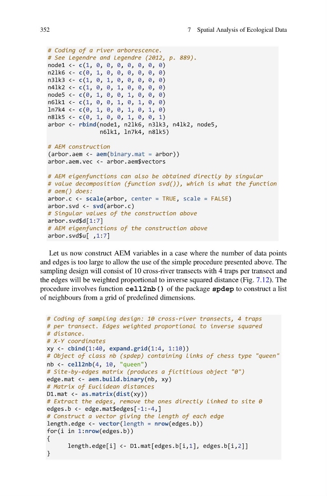
# Coding of a river arborescence.
# See Legendre and Legendre (2012, p. 889).
node1 <- c(1, 0, 0, 0, 0, 0, 0, 0)
n2lk6 <- c(0, 1, 0, 0, 0, 0, 0, 0)
n3lk3 <- c(1, 0, 1, 0, 0, 0, 0, 0)
n4lk2 <- c(1, 0, 0, 1, 0, 0, 0, 0)
node5 <- c(0, 1, 0, 0, 1, 0, 0, 0)
n6lk1 <- c(1, 0, 0, 1, 0, 1, 0, 0)
ln7k4 <- c(0, 1, 0, 0, 1, 0, 1, 0)
n8lk5 <- c(0, 1, 0, 0, 1, 0, 0, 1)
arbor <- rbind(node1, n2lk6, n3lk3, n4lk2, node5,
n6lk1, ln7k4, n8lk5)
# AEM construction
(arbor.aem <- aem(binary.mat = arbor))
arbor.aem.vec <- arbor.aem$vectors
# AEM eigenfunctions can also be obtained directly by singular
# value decomposition (function svd()), which is what the function
# aem() does:
arbor.c <- scale(arbor, center = TRUE, scale = FALSE)
arbor.svd <- svd(arbor.c)
# Singular values of the construction above
arbor.svd$d[1:7]
# AEM eigenfunctions of the construction above
arbor.svd$u[ ,1:7]
Let us now construct AEM variables in a case where the number of data points
and edges is too large to allow the use of the simple procedure presented above. The
sampling design will consist of 10 cross-river transects with 4 traps per transect and
the edges will be weighted proportional to inverse squared distance (Fig. 7.12). The
procedure involves function cell2nb() of the package spdep to construct a list
of neighbours from a grid of predefined dimensions.
# Coding of sampling design: 10 cross-river transects, 4 traps
# per transect. Edges weighted proportional to inverse squared
# distance.
# X-Y coordinates
xy <- cbind(1:40, expand.grid(1:4, 1:10))
# Object of class nb (spdep) containing links of chess type "queen"
nb <- cell2nb(4, 10, "queen")
# Site-by-edges matrix (produces a fictitious object "0")
edge.mat <- aem.build.binary(nb, xy)
# Matrix of Euclidean distances
D1.mat <- as.matrix(dist(xy))
# Extract the edges, remove the ones directly linked to site 0
edges.b <- edge.mat$edges[-1:-4,]
# Construct a vector giving the length of each edge
length.edge <- vector(length = nrow(edges.b))
for(i in 1:nrow(edges.b))
{
length.edge[i] <- D1.mat[edges.b[i,1], edges.b[i,2]]
}
352
7 Spatial Analysis of Ecological Data
# See Legendre and Legendre (2012, p. 889).
node1 <- c(1, 0, 0, 0, 0, 0, 0, 0)
n2lk6 <- c(0, 1, 0, 0, 0, 0, 0, 0)
n3lk3 <- c(1, 0, 1, 0, 0, 0, 0, 0)
n4lk2 <- c(1, 0, 0, 1, 0, 0, 0, 0)
node5 <- c(0, 1, 0, 0, 1, 0, 0, 0)
n6lk1 <- c(1, 0, 0, 1, 0, 1, 0, 0)
ln7k4 <- c(0, 1, 0, 0, 1, 0, 1, 0)
n8lk5 <- c(0, 1, 0, 0, 1, 0, 0, 1)
arbor <- rbind(node1, n2lk6, n3lk3, n4lk2, node5,
n6lk1, ln7k4, n8lk5)
# AEM construction
(arbor.aem <- aem(binary.mat = arbor))
arbor.aem.vec <- arbor.aem$vectors
# AEM eigenfunctions can also be obtained directly by singular
# value decomposition (function svd()), which is what the function
# aem() does:
arbor.c <- scale(arbor, center = TRUE, scale = FALSE)
arbor.svd <- svd(arbor.c)
# Singular values of the construction above
arbor.svd$d[1:7]
# AEM eigenfunctions of the construction above
arbor.svd$u[ ,1:7]
Let us now construct AEM variables in a case where the number of data points
and edges is too large to allow the use of the simple procedure presented above. The
sampling design will consist of 10 cross-river transects with 4 traps per transect and
the edges will be weighted proportional to inverse squared distance (Fig. 7.12). The
procedure involves function cell2nb() of the package spdep to construct a list
of neighbours from a grid of predefined dimensions.
# Coding of sampling design: 10 cross-river transects, 4 traps
# per transect. Edges weighted proportional to inverse squared
# distance.
# X-Y coordinates
xy <- cbind(1:40, expand.grid(1:4, 1:10))
# Object of class nb (spdep) containing links of chess type "queen"
nb <- cell2nb(4, 10, "queen")
# Site-by-edges matrix (produces a fictitious object "0")
edge.mat <- aem.build.binary(nb, xy)
# Matrix of Euclidean distances
D1.mat <- as.matrix(dist(xy))
# Extract the edges, remove the ones directly linked to site 0
edges.b <- edge.mat$edges[-1:-4,]
# Construct a vector giving the length of each edge
length.edge <- vector(length = nrow(edges.b))
for(i in 1:nrow(edges.b))
{
length.edge[i] <- D1.mat[edges.b[i,1], edges.b[i,2]]
}
352
7 Spatial Analysis of Ecological Data