

# 1. Test trend
mite.XY.rda <- rda(mite.h, mite.xy)
anova(mite.XY.rda)
# 2. Test and forward selection of the environmental variables
# Recode environmental variables 3 to 5 into dummy binary variables
substrate <- model.matrix( ~ mite.env[ ,3])[ ,-1]
shrubs <- model.matrix( ~ mite.env[ ,4])[ ,-1]
topography <- model.matrix( ~ mite.env[ ,5])[ ,-1]
mite.env2 <- cbind(mite.env[ ,1:2], substrate, shrubs, topography)
colnames(mite.env2)
"topography")
# Forward selection of the environmental variables
mite.env.rda <- rda(mite.h ~., mite.env2)
(mite.env.R2a <- RsquareAdj(mite.env.rda)$adj.r.squared)
mite.env.fwd
nperm = 9999)
env.sign <- sort(mite.env.fwd$order)
env.red <- mite.env2[ ,c(env.sign)]
colnames(env.red)
# 3. Test and forward selection of the dbMEM variables
# Run the global dbMEM analysis on the *detrended* mite data
mite.det.dbmem.rda <- rda(mite.h.det ~., mite.dbmem)
anova(mite.det.dbmem.rda)
# Since the analysis is significant, compute the adjusted R2
# and run a forward selection of the dbMEM variables
(mite.det.dbmem.R2a
X2
X3
X4
[a]
[b]
[c]
[d]
[e]
[f]
[g]
[h]
[i]
[j]
[k]
[l]
[m]
[n]
[o]
Residuals = [p]
X1
X2
X3
X4
0.073
0.037
0.070
0.016
0.274
0.080
0.034
0.002
0.002
Residuals = 0.475
Values <0 not shown
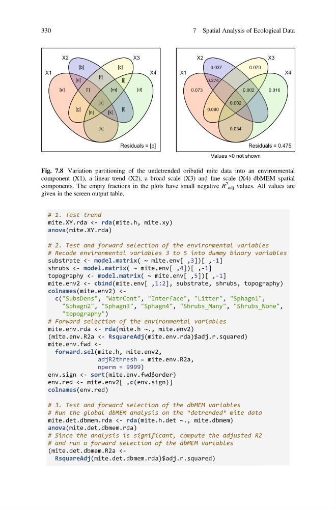
Fig. 7.8 Variation partitioning of the undetrended oribatid mite data into an environmental
component (X1), a linear trend (X2), a broad scale (X3) and fine scale (X4) dbMEM spatial
components. The empty fractions in the plots have small negative R
2
adj values. All values are
given in the screen output table.
330
7 Spatial Analysis of Ecological Data
mite.XY.rda <- rda(mite.h, mite.xy)
anova(mite.XY.rda)
# 2. Test and forward selection of the environmental variables
# Recode environmental variables 3 to 5 into dummy binary variables
substrate <- model.matrix( ~ mite.env[ ,3])[ ,-1]
shrubs <- model.matrix( ~ mite.env[ ,4])[ ,-1]
topography <- model.matrix( ~ mite.env[ ,5])[ ,-1]
mite.env2 <- cbind(mite.env[ ,1:2], substrate, shrubs, topography)
colnames(mite.env2)
"topography")
# Forward selection of the environmental variables
mite.env.rda <- rda(mite.h ~., mite.env2)
(mite.env.R2a <- RsquareAdj(mite.env.rda)$adj.r.squared)
mite.env.fwd
nperm = 9999)
env.sign <- sort(mite.env.fwd$order)
env.red <- mite.env2[ ,c(env.sign)]
colnames(env.red)
# 3. Test and forward selection of the dbMEM variables
# Run the global dbMEM analysis on the *detrended* mite data
mite.det.dbmem.rda <- rda(mite.h.det ~., mite.dbmem)
anova(mite.det.dbmem.rda)
# Since the analysis is significant, compute the adjusted R2
# and run a forward selection of the dbMEM variables
(mite.det.dbmem.R2a
X2
X3
X4
[a]
[b]
[c]
[d]
[e]
[f]
[g]
[h]
[i]
[j]
[k]
[l]
[m]
[n]
[o]
Residuals = [p]
X1
X2
X3
X4
0.073
0.037
0.070
0.016
0.274
0.080
0.034
0.002
0.002
Residuals = 0.475
Values <0 not shown
Fig. 7.8 Variation partitioning of the undetrended oribatid mite data into an environmental
component (X1), a linear trend (X2), a broad scale (X3) and fine scale (X4) dbMEM spatial
components. The empty fractions in the plots have small negative R
2
adj values. All values are
given in the screen output table.
330
7 Spatial Analysis of Ecological Data