

response data on the X-Y coordinates of the sampling sites. Of course, this will only
model a linear trend; a plane will be fitted through the data in the same way as a
straight line would be fitted to data collected along a transect by regressing them on
their X coordinates.
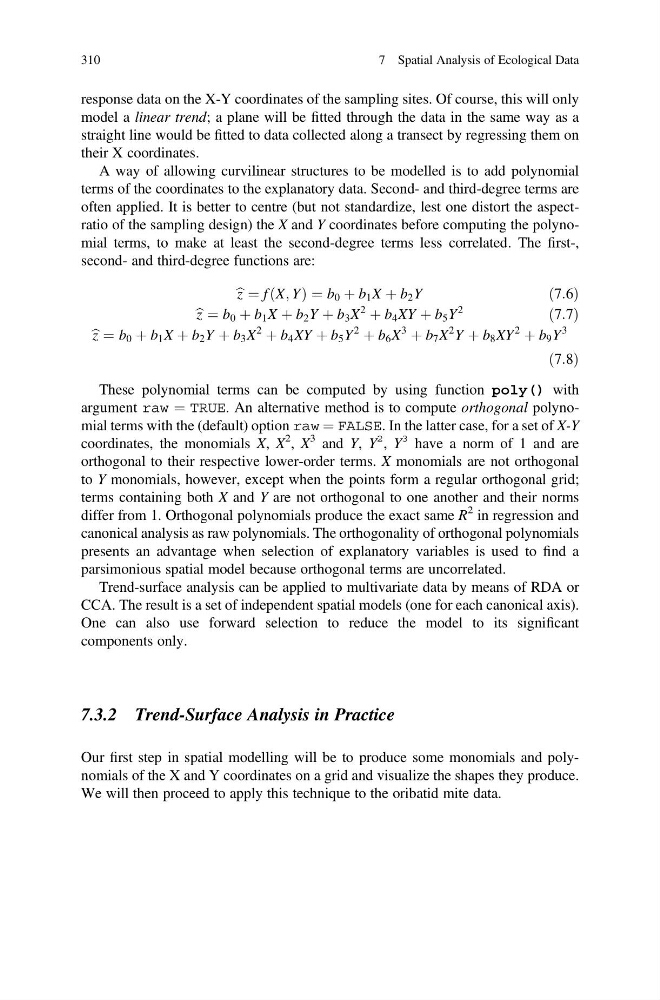
A way of allowing curvilinear structures to be modelled is to add polynomial
terms of the coordinates to the explanatory data. Second- and third-degree terms are
often applied. It is better to centre (but not standardize, lest one distort the aspectratio of the sampling design) the X and Y coordinates before computing the polynomial terms, to make at least the second-degree terms less correlated. The first-,
second- and third-degree functions are:
b z ¼ f X; Y
ð
Þ ¼ b 0 þ b 1 X þ b 2 Y
ð7:6Þ
b z ¼ b 0 þ b 1 X þ b 2 Y þ b 3 X
2
þ b 4 XY þ b 5 Y
2
ð7:7Þ
b z ¼ b 0 þ b 1 X þ b 2 Y þ b 3 X
2
þ b 4 XY þ b 5 Y
2
þ b 6 X
3
þ b 7 X
2 Y þ b 8 XY
2
þ b 9 Y
3
ð7:8Þ
These polynomial terms can be computed by using function poly() with
argument raw ¼ TRUE. An alternative method is to compute orthogonal polynomial terms with the (default) option raw ¼ FALSE. In the latter case, for a set of X-Y
coordinates, the monomials X, X
2 , X
3 and Y, Y
2
, Y
3 have a norm of 1 and are
orthogonal to their respective lower-order terms. X monomials are not orthogonal
to Y monomials, however, except when the points form a regular orthogonal grid;
terms containing both X and Y are not orthogonal to one another and their norms
differ from 1. Orthogonal polynomials produce the exact same R
2 in regression and
canonical analysis as raw polynomials. The orthogonality of orthogonal polynomials
presents an advantage when selection of explanatory variables is used to find a
parsimonious spatial model because orthogonal terms are uncorrelated.
Trend-surface analysis can be applied to multivariate data by means of RDA or
CCA. The result is a set of independent spatial models (one for each canonical axis).
One can also use forward selection to reduce the model to its significant
components only.
7.3.2 Trend-Surface Analysis in Practice
Our first step in spatial modelling will be to produce some monomials and polynomials of the X and Y coordinates on a grid and visualize the shapes they produce.
We will then proceed to apply this technique to the oribatid mite data.
310
7 Spatial Analysis of Ecological Data
model a linear trend; a plane will be fitted through the data in the same way as a
straight line would be fitted to data collected along a transect by regressing them on
their X coordinates.
A way of allowing curvilinear structures to be modelled is to add polynomial
terms of the coordinates to the explanatory data. Second- and third-degree terms are
often applied. It is better to centre (but not standardize, lest one distort the aspectratio of the sampling design) the X and Y coordinates before computing the polynomial terms, to make at least the second-degree terms less correlated. The first-,
second- and third-degree functions are:
b z ¼ f X; Y
ð
Þ ¼ b 0 þ b 1 X þ b 2 Y
ð7:6Þ
b z ¼ b 0 þ b 1 X þ b 2 Y þ b 3 X
2
þ b 4 XY þ b 5 Y
2
ð7:7Þ
b z ¼ b 0 þ b 1 X þ b 2 Y þ b 3 X
2
þ b 4 XY þ b 5 Y
2
þ b 6 X
3
þ b 7 X
2 Y þ b 8 XY
2
þ b 9 Y
3
ð7:8Þ
These polynomial terms can be computed by using function poly() with
argument raw ¼ TRUE. An alternative method is to compute orthogonal polynomial terms with the (default) option raw ¼ FALSE. In the latter case, for a set of X-Y
coordinates, the monomials X, X
2 , X
3 and Y, Y
2
, Y
3 have a norm of 1 and are
orthogonal to their respective lower-order terms. X monomials are not orthogonal
to Y monomials, however, except when the points form a regular orthogonal grid;
terms containing both X and Y are not orthogonal to one another and their norms
differ from 1. Orthogonal polynomials produce the exact same R
2 in regression and
canonical analysis as raw polynomials. The orthogonality of orthogonal polynomials
presents an advantage when selection of explanatory variables is used to find a
parsimonious spatial model because orthogonal terms are uncorrelated.
Trend-surface analysis can be applied to multivariate data by means of RDA or
CCA. The result is a set of independent spatial models (one for each canonical axis).
One can also use forward selection to reduce the model to its significant
components only.
7.3.2 Trend-Surface Analysis in Practice
Our first step in spatial modelling will be to produce some monomials and polynomials of the X and Y coordinates on a grid and visualize the shapes they produce.
We will then proceed to apply this technique to the oribatid mite data.
310
7 Spatial Analysis of Ecological Data