

When the data set covers a sufficiently large area, it is possible to project the sites
onto a Google Maps® map:
## Sites projected onto a Google Maps® background
# By default the plot method of the googleVis package uses
# the standard browser to display its output.
nom <- latlong$Site
latlong2 <- paste(latlong$LatitudeN, latlong$LongitudeE, sep = ":")
df <- data.frame(latlong2, nom, stringsAsFactors = FALSE)
mymap1 <- gvisMap(df,
locationvar = "latlong2",
tipvar = "nom",
options = list(showTip = TRUE)
)
plot(mymap1)
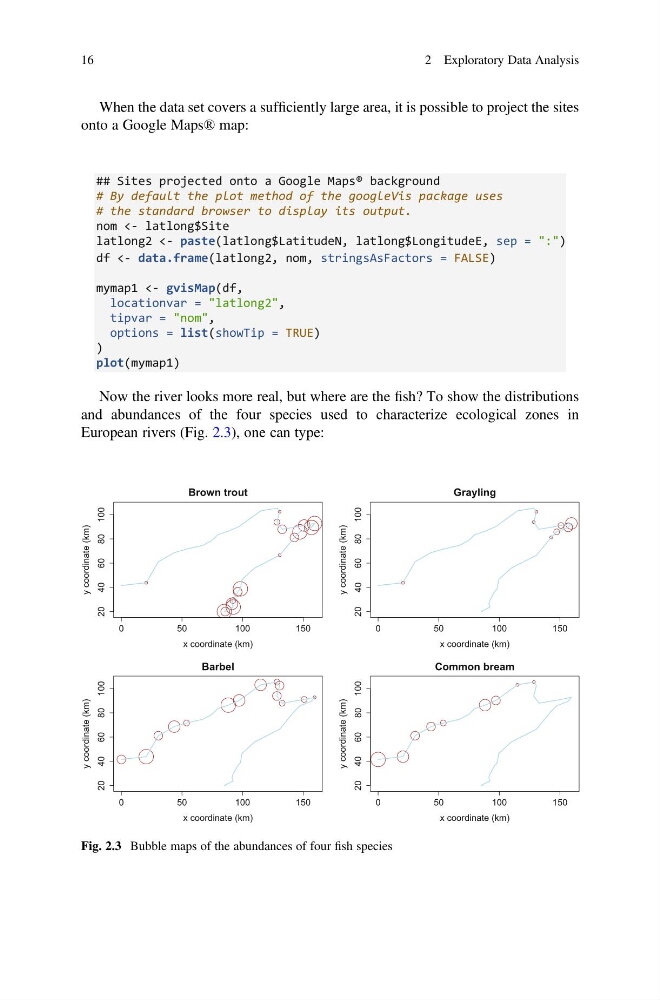
Now the river looks more real, but where are the fish? To show the distributions
and abundances of the four species used to characterize ecological zones in
European rivers (Fig. 2.3), one can type:
0
50
100
150
20
40
60
80 100
Brown trout
x coordinate (km)
y coordinate (km)
0
50
100
150
20
40
60
80 100
Grayling
x coordinate (km)
y coordinate (km)
0
50
100
150
20
40
60
80 100
Barbel
x coordinate (km)
y coordinate (km)
0
50
100
150
20
40
60
80 100
Common bream
x coordinate (km)
y coordinate (km)
Fig. 2.3 Bubble maps of the abundances of four fish species
16
2 Exploratory Data Analysis
onto a Google Maps® map:
## Sites projected onto a Google Maps® background
# By default the plot method of the googleVis package uses
# the standard browser to display its output.
nom <- latlong$Site
latlong2 <- paste(latlong$LatitudeN, latlong$LongitudeE, sep = ":")
df <- data.frame(latlong2, nom, stringsAsFactors = FALSE)
mymap1 <- gvisMap(df,
locationvar = "latlong2",
tipvar = "nom",
options = list(showTip = TRUE)
)
plot(mymap1)
Now the river looks more real, but where are the fish? To show the distributions
and abundances of the four species used to characterize ecological zones in
European rivers (Fig. 2.3), one can type:
0
50
100
150
20
40
60
80 100
Brown trout
x coordinate (km)
y coordinate (km)
0
50
100
150
20
40
60
80 100
Grayling
x coordinate (km)
y coordinate (km)
0
50
100
150
20
40
60
80 100
Barbel
x coordinate (km)
y coordinate (km)
0
50
100
150
20
40
60
80 100
Common bream
x coordinate (km)
y coordinate (km)
Fig. 2.3 Bubble maps of the abundances of four fish species
16
2 Exploratory Data Analysis