

(preliminary use of ordination functions to obtain the data, transformed or not), a
PCA of the standardized data (correlation matrix) is first performed on each of the
two data tables. The proportion of variance accounted for by the axes is then
computed to assess the number of axes to be retained in the CoIA. In this example,
3 axes of the chemistry PCA account for 89.8% variation, and 2 axes of the
physiography PCA account for 98.9% variation. After having verified that the row
weights are equal in the two PCAs, these two results are then submitted to CoIA,
which is asked to retain two canonical axes. A permutation test is run to assess the
significance of the co-inertia structure of the data tables.
# PCA on both matrices using ade4 functions
dudi.chem <- dudi.pca(envchem2,
scale = TRUE,
scannf = FALSE)
dudi.topo <- dudi.pca(envtopo2,
scale = TRUE,
scannf = FALSE)
# Cumulated relative variation of eigenvalues
cumsum(dudi.chem$eig / sum(dudi.chem$eig))
# Cumulated relative variation of eigenvalues
cumsum(dudi.topo$eig / sum(dudi.topo$eig))
# Are the row weights equal in the 2 analyses?
all.equal(dudi.chem$lw, dudi.topo$lw)
# Co-inertia analysis
coia.chem.topo
nf = 2)
summary(coia.chem.topo)
# Relative variation on first eigenvalue
coia.chem.topo$eig[1] / sum(coia.chem.topo$eig)
# Permutation test
randtest(coia.chem.topo, nrepet = 999)
# Plot results
plot(coia.chem.topo)
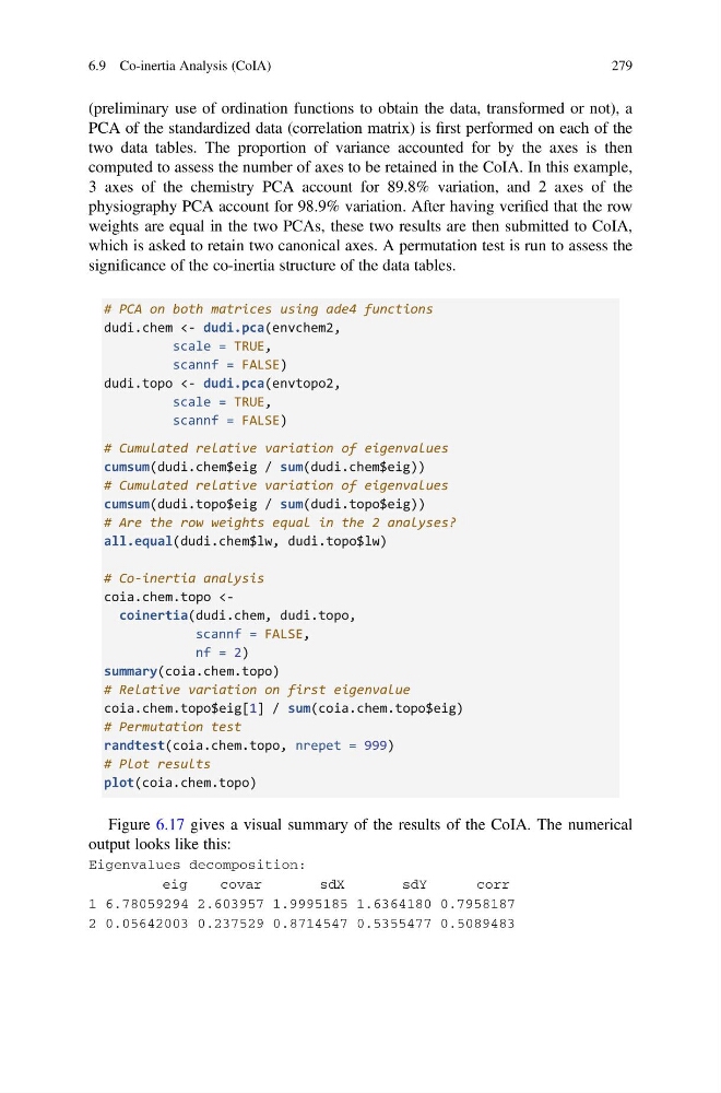
Figure 6.17 gives a visual summary of the results of the CoIA. The numerical
output looks like this:
Eigenvalues decomposition:
eig
covar
sdX
sdY
corr
1 6.78059294 2.603957 1.9995185 1.6364180 0.7958187
2 0.05642003 0.237529 0.8714547 0.5355477 0.5089483
6.9 Co-inertia Analysis (CoIA)
279
PCA of the standardized data (correlation matrix) is first performed on each of the
two data tables. The proportion of variance accounted for by the axes is then
computed to assess the number of axes to be retained in the CoIA. In this example,
3 axes of the chemistry PCA account for 89.8% variation, and 2 axes of the
physiography PCA account for 98.9% variation. After having verified that the row
weights are equal in the two PCAs, these two results are then submitted to CoIA,
which is asked to retain two canonical axes. A permutation test is run to assess the
significance of the co-inertia structure of the data tables.
# PCA on both matrices using ade4 functions
dudi.chem <- dudi.pca(envchem2,
scale = TRUE,
scannf = FALSE)
dudi.topo <- dudi.pca(envtopo2,
scale = TRUE,
scannf = FALSE)
# Cumulated relative variation of eigenvalues
cumsum(dudi.chem$eig / sum(dudi.chem$eig))
# Cumulated relative variation of eigenvalues
cumsum(dudi.topo$eig / sum(dudi.topo$eig))
# Are the row weights equal in the 2 analyses?
all.equal(dudi.chem$lw, dudi.topo$lw)
# Co-inertia analysis
coia.chem.topo
nf = 2)
summary(coia.chem.topo)
# Relative variation on first eigenvalue
coia.chem.topo$eig[1] / sum(coia.chem.topo$eig)
# Permutation test
randtest(coia.chem.topo, nrepet = 999)
# Plot results
plot(coia.chem.topo)
Figure 6.17 gives a visual summary of the results of the CoIA. The numerical
output looks like this:
Eigenvalues decomposition:
eig
covar
sdX
sdY
corr
1 6.78059294 2.603957 1.9995185 1.6364180 0.7958187
2 0.05642003 0.237529 0.8714547 0.5355477 0.5089483
6.9 Co-inertia Analysis (CoIA)
279