

# Biplot scores of explanatory variables
coordX <- corXZ %*% D
# Scaling 1
coordX2 <- corXZ
# Scaling 2
row.names(coordX) <- colnames(X)
row.names(coordX2) <- colnames(X)
# Scaling to sqrt of the relative eigenvalue
# (for scaling 2)
U2 <- U %*% diag(sqrt(ev))
row.names(U2) <- colnames(Y)
F2 <- F %*% diag(1/sqrt(ev))
row.names(F2) <- row.names(Y)
Z2 <- Z %*% diag(1/sqrt(ev))
row.names(Z2) <- row.names(Y)
# Unadjusted R2
R2 <- sum(ev/trace)
# Adjusted R2
R2a <- 1 - ((n - 1)/(n - m - 1)) * (1 - R2)
# 4. PCA on residuals
# Write your own code as in Chapter 5. It could begin
# with :
#
eigenSres <- eigen(cov(Yres))
#
evr <- eigenSres$values
# 5. Output
result
names(result)
"Biplot_sc1", "Species_sc2", "wa_sc2", "lc_sc2",
"Biplot_sc2")
result
}
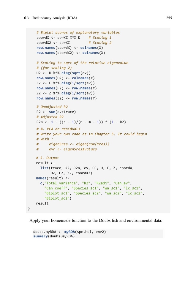
Apply your homemade function to the Doubs fish and environmental data:
doubs.myRDA <- myRDA(spe.hel, env2)
summary(doubs.myRDA)
6.3 Redundancy Analysis (RDA)
255
coordX <- corXZ %*% D
# Scaling 1
coordX2 <- corXZ
# Scaling 2
row.names(coordX) <- colnames(X)
row.names(coordX2) <- colnames(X)
# Scaling to sqrt of the relative eigenvalue
# (for scaling 2)
U2 <- U %*% diag(sqrt(ev))
row.names(U2) <- colnames(Y)
F2 <- F %*% diag(1/sqrt(ev))
row.names(F2) <- row.names(Y)
Z2 <- Z %*% diag(1/sqrt(ev))
row.names(Z2) <- row.names(Y)
# Unadjusted R2
R2 <- sum(ev/trace)
# Adjusted R2
R2a <- 1 - ((n - 1)/(n - m - 1)) * (1 - R2)
# 4. PCA on residuals
# Write your own code as in Chapter 5. It could begin
# with :
#
eigenSres <- eigen(cov(Yres))
#
evr <- eigenSres$values
# 5. Output
result
names(result)
"Biplot_sc1", "Species_sc2", "wa_sc2", "lc_sc2",
"Biplot_sc2")
result
}
Apply your homemade function to the Doubs fish and environmental data:
doubs.myRDA <- myRDA(spe.hel, env2)
summary(doubs.myRDA)
6.3 Redundancy Analysis (RDA)
255