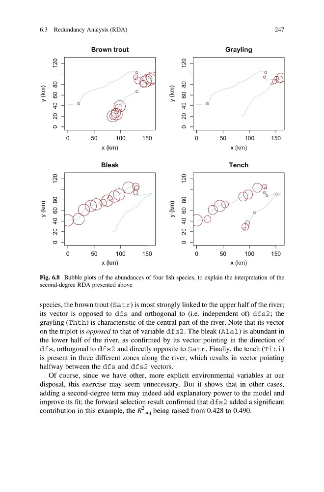
species, the brown trout (Satr) is most strongly linked to the upper half of the river;
its vector is opposed to dfs and orthogonal to (i.e. independent of) dfs2; the
grayling (Thth) is characteristic of the central part of the river. Note that its vector
on the triplot is opposed to that of variable dfs2. The bleak (Alal) is abundant in
the lower half of the river, as confirmed by its vector pointing in the direction of
dfs, orthogonal to dfs2 and directly opposite to Satr. Finally, the tench (Titi)
is present in three different zones along the river, which results in vector pointing
halfway between the dfs and dfs2 vectors.
Of course, since we have other, more explicit environmental variables at our
disposal, this exercise may seem unnecessary. But it shows that in other cases,
adding a second-degree term may indeed add explanatory power to the model and
improve its fit; the forward selection result confirmed that dfs2 added a significant
contribution in this example, the R
2
adj being raised from 0.428 to 0.490.
0
50
100
150
0 20 40 60 80
120
Brown trout
x (km)
y (km)
0
50
100
150
0 20
40 60
80
120
Grayling
x (km)
y (km)
0
50
100
150
0 20 40 60 80
120
Bleak
x (km)
y (km)
0
50
100
150
0 20 40
60 80
120
Tench
x (km)
y (km)
Fig. 6.8 Bubble plots of the abundances of four fish species, to explain the interpretation of the
second-degree RDA presented above
6.3 Redundancy Analysis (RDA)
247