

RDA. The first one involves a single explanatory variable and shows the effect of
incorporating a second-degree term into the model. The second example proposes a
full RDA with all explanatory variables (except dfs) and their second-degree terms,
followed by forward selection.
A single explanatory variable
In the Doubs data, there are several species that are found mostly in the central
section of the river. Their relationship with the variable “distance from the source”
(dfs) is therefore unimodal: absence first, then presence, then absence again. Such a
simple case could be a good candidate to experiment with a second-degree polynomial, i.e. a sum of terms encompassing a variable to exponents 1 and 2. When
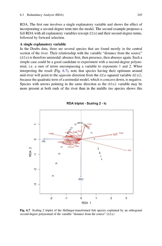
interpreting the result (Fig. 6.7), note that species having their optimum around
mid-river will point to the opposite direction from the dfs-squared variable dfs2,
because the quadratic term of a unimodal model, which is concave down, is negative.
Species with arrows pointing in the same direction as the dfs2 variable may be
more present at both ends of the river than in the middle (no species shows this
-2
-1
0
1
2
3
-3
-2
-1
0
1
RDA triplot - Scaling 2 - lc
RDA 1
RDA 2
1
2
3
4
5
6
7
9
10
11
12
13
14
15
16
17
18
19
20
21
22
23
24
25
26
27
28
29
30
Cogo
Satr
Phph
Babl
Thth
Teso
Chna
Pato
Lele
Sqce
Baba
Albi
Gogo
Eslu
Pefl
Rham
Legi
Scer
Cyca
Titi
Abbr
Icme
Gyce
Ruru
Blbj
Alal
Anan
dfs
dfs2
Fig. 6.7 Scaling 2 triplot of the Hellinger-transformed fish species explained by an orthogonal
second-degree polynomial of the variable “distance from the source” (dfs)
6.3 Redundancy Analysis (RDA)
245
incorporating a second-degree term into the model. The second example proposes a
full RDA with all explanatory variables (except dfs) and their second-degree terms,
followed by forward selection.
A single explanatory variable
In the Doubs data, there are several species that are found mostly in the central
section of the river. Their relationship with the variable “distance from the source”
(dfs) is therefore unimodal: absence first, then presence, then absence again. Such a
simple case could be a good candidate to experiment with a second-degree polynomial, i.e. a sum of terms encompassing a variable to exponents 1 and 2. When
interpreting the result (Fig. 6.7), note that species having their optimum around
mid-river will point to the opposite direction from the dfs-squared variable dfs2,
because the quadratic term of a unimodal model, which is concave down, is negative.
Species with arrows pointing in the same direction as the dfs2 variable may be
more present at both ends of the river than in the middle (no species shows this
-2
-1
0
1
2
3
-3
-2
-1
0
1
RDA triplot - Scaling 2 - lc
RDA 1
RDA 2
1
2
3
4
5
6
7
9
10
11
12
13
14
15
16
17
18
19
20
21
22
23
24
25
26
27
28
29
30
Cogo
Satr
Phph
Babl
Thth
Teso
Chna
Pato
Lele
Sqce
Baba
Albi
Gogo
Eslu
Pefl
Rham
Legi
Scer
Cyca
Titi
Abbr
Icme
Gyce
Ruru
Blbj
Alal
Anan
dfs
dfs2
Fig. 6.7 Scaling 2 triplot of the Hellinger-transformed fish species explained by an orthogonal
second-degree polynomial of the variable “distance from the source” (dfs)
6.3 Redundancy Analysis (RDA)
245