

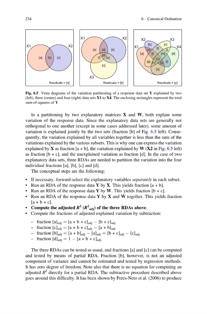
In a partitioning by two explanatory matrices X and W, both explain some
variation of the response data. Since the explanatory data sets are generally not
orthogonal to one another (except in some cases addressed later), some amount of
variation is explained jointly by the two sets (fraction [b] of Fig. 6.5 left). Consequently, the variation explained by all variables together is less than the sum of the
variations explained by the various subsets. This is why one can express the variation
explained by X as fraction [a + b], the variation explained by W (X2 in Fig. 6.5 left)
as fraction [b + c], and the unexplained variation as fraction [d]. In the case of two
explanatory data sets, three RDAs are needed to partition the variation into the four
individual fractions [a], [b], [c] and [d].
The conceptual steps are the following:
• If necessary, forward-select the explanatory variables separately in each subset.
• Run an RDA of the response data Y by X. This yields fraction [a + b].
• Run an RDA of the response data Y by W. This yields fraction [b + c].
• Run an RDA of the response data Y by X and W together. This yields fraction
[a + b + c].
• Compute the adjusted R
2 (R
2
adj ) of the three RDAs above.
• Compute the fractions of adjusted explained variation by subtraction:
– fraction [a] adj ¼ [a + b + c] adj À [b + c] adj
– fraction [c] adj ¼ [a + b + c] adj À [a + b] adj
– fraction [b] adj ¼ [a + b] adj À [a] adj ¼ [b + c] adj À [c] adj
– fraction [d] adj ¼ 1 À [a + b + c] adj
The three RDAs can be tested as usual, and fractions [a] and [c] can be computed
and tested by means of partial RDA. Fraction [b], however, is not an adjusted
component of variance and cannot be estimated and tested by regression methods.
It has zero degree of freedom. Note also that there is no equation for computing an
adjusted R
2 directly for a partial RDA. The subtractive procedure described above
goes around this difficulty. It has been shown by Peres-Neto et al. (2006) to produce
X1
X2
[a]
[b]
[c]
Residuals = [d]
X1
X2
X3
[a]
[b]
[c]
[d]
[e]
[f]
[g]
Residuals = [h]
X1
X2
X3
X4
[a]
[b]
[c]
[d]
[e]
[f]
[g]
[h]
[i]
[j]
[k]
[l]
[m]
[n]
[o]
Residuals = [p]
Fig. 6.5 Venn diagrams of the variation partitioning of a response data set Y explained by two
(left), three (centre) and four (right) data sets X1 to X4. The enclosing rectangles represent the total
sum-of-squares of Y
234
6 Canonical Ordination
variation of the response data. Since the explanatory data sets are generally not
orthogonal to one another (except in some cases addressed later), some amount of
variation is explained jointly by the two sets (fraction [b] of Fig. 6.5 left). Consequently, the variation explained by all variables together is less than the sum of the
variations explained by the various subsets. This is why one can express the variation
explained by X as fraction [a + b], the variation explained by W (X2 in Fig. 6.5 left)
as fraction [b + c], and the unexplained variation as fraction [d]. In the case of two
explanatory data sets, three RDAs are needed to partition the variation into the four
individual fractions [a], [b], [c] and [d].
The conceptual steps are the following:
• If necessary, forward-select the explanatory variables separately in each subset.
• Run an RDA of the response data Y by X. This yields fraction [a + b].
• Run an RDA of the response data Y by W. This yields fraction [b + c].
• Run an RDA of the response data Y by X and W together. This yields fraction
[a + b + c].
• Compute the adjusted R
2 (R
2
adj ) of the three RDAs above.
• Compute the fractions of adjusted explained variation by subtraction:
– fraction [a] adj ¼ [a + b + c] adj À [b + c] adj
– fraction [c] adj ¼ [a + b + c] adj À [a + b] adj
– fraction [b] adj ¼ [a + b] adj À [a] adj ¼ [b + c] adj À [c] adj
– fraction [d] adj ¼ 1 À [a + b + c] adj
The three RDAs can be tested as usual, and fractions [a] and [c] can be computed
and tested by means of partial RDA. Fraction [b], however, is not an adjusted
component of variance and cannot be estimated and tested by regression methods.
It has zero degree of freedom. Note also that there is no equation for computing an
adjusted R
2 directly for a partial RDA. The subtractive procedure described above
goes around this difficulty. It has been shown by Peres-Neto et al. (2006) to produce
X1
X2
[a]
[b]
[c]
Residuals = [d]
X1
X2
X3
[a]
[b]
[c]
[d]
[e]
[f]
[g]
Residuals = [h]
X1
X2
X3
X4
[a]
[b]
[c]
[d]
[e]
[f]
[g]
[h]
[i]
[j]
[k]
[l]
[m]
[n]
[o]
Residuals = [p]
Fig. 6.5 Venn diagrams of the variation partitioning of a response data set Y explained by two
(left), three (centre) and four (right) data sets X1 to X4. The enclosing rectangles represent the total
sum-of-squares of Y
234
6 Canonical Ordination