

(spe.rda.pars <- rda(spe.hel ~ ele + oxy + bod, data = env2))
anova(spe.rda.pars, permutations = how(nperm = 999))
anova(spe.rda.pars, permutations = how(nperm = 999), by = "axis")
(R2a.pars <- RsquareAdj(spe.rda.pars)$adj.r.squared)
# Compare the variance inflation factors
vif.cca(spe.rda.all)
vif.cca(spe.rda.pars)
These results are fascinating in that they demonstrate how a parsimonious
approach can help improve the quality of a model. With a moderate cost in
explanatory power, we produced a model that is as highly significant, has no harmful
collinearity (all VIFs are now well below 10), and can be decomposed into three
significant canonical axes, whereas the global model produced only two
significant axes.
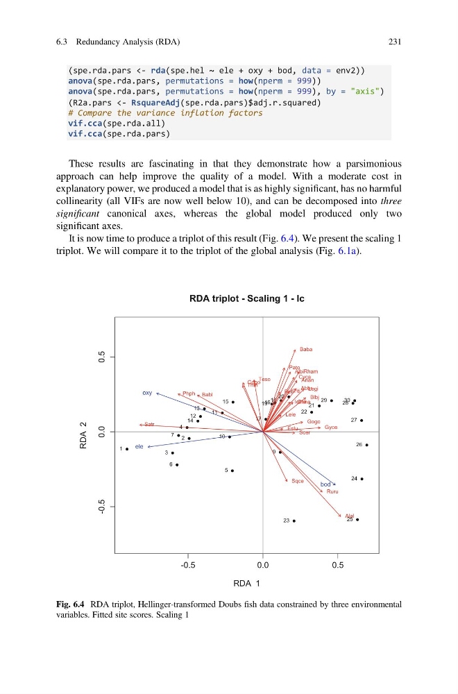
It is now time to produce a triplot of this result (Fig. 6.4). We present the scaling 1
triplot. We will compare it to the triplot of the global analysis (Fig. 6.1a).
-0.5
0.0
0.5
-0.5
0.0
0.5
RDA triplot - Scaling 1 - lc
RDA 1
RDA 2
1
2
3
4
5
6
7
9
10
11
12
13
14
15
16
17
18
19
20
21
22
23
24
25
26
27
28
29
30
Cogo
Satr
Phph Babl
Thth
Teso
Chna
Pato
Lele
Sqce
Baba
Albi
Gogo
Eslu
Pefl
Rham
Legi
Scer
Cyca
Titi
Abbr
Icme
Gyce
Ruru
Blbj
Alal
Anan
ele
oxy
bod
Fig. 6.4 RDA triplot, Hellinger-transformed Doubs fish data constrained by three environmental
variables. Fitted site scores. Scaling 1
6.3 Redundancy Analysis (RDA)
231
anova(spe.rda.pars, permutations = how(nperm = 999))
anova(spe.rda.pars, permutations = how(nperm = 999), by = "axis")
(R2a.pars <- RsquareAdj(spe.rda.pars)$adj.r.squared)
# Compare the variance inflation factors
vif.cca(spe.rda.all)
vif.cca(spe.rda.pars)
These results are fascinating in that they demonstrate how a parsimonious
approach can help improve the quality of a model. With a moderate cost in
explanatory power, we produced a model that is as highly significant, has no harmful
collinearity (all VIFs are now well below 10), and can be decomposed into three
significant canonical axes, whereas the global model produced only two
significant axes.
It is now time to produce a triplot of this result (Fig. 6.4). We present the scaling 1
triplot. We will compare it to the triplot of the global analysis (Fig. 6.1a).
-0.5
0.0
0.5
-0.5
0.0
0.5
RDA triplot - Scaling 1 - lc
RDA 1
RDA 2
1
2
3
4
5
6
7
9
10
11
12
13
14
15
16
17
18
19
20
21
22
23
24
25
26
27
28
29
30
Cogo
Satr
Phph Babl
Thth
Teso
Chna
Pato
Lele
Sqce
Baba
Albi
Gogo
Eslu
Pefl
Rham
Legi
Scer
Cyca
Titi
Abbr
Icme
Gyce
Ruru
Blbj
Alal
Anan
ele
oxy
bod
Fig. 6.4 RDA triplot, Hellinger-transformed Doubs fish data constrained by three environmental
variables. Fitted site scores. Scaling 1
6.3 Redundancy Analysis (RDA)
231