# Compute matrix U2 (to represent variables in scaling 2 plots)
# eq. 9.8
U2 <- U %*% diag(Y.eig$values ^ 0.5)
rownames(U2) <- var.names
# Compute matrix G (to represent objects in scaling 2 plots)
# eq. 9.14
G <- F %*% diag(Y.eig$values ^ 0.5)
rownames(G) <- object.names
# Output of a list containing all the results
result <- list(Y.eig$values, U, F, U2, G)
names(result) <- c("eigenvalues", "U", "F", "U2", "G")
result
}
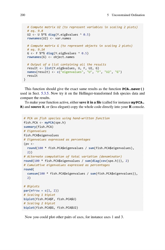
This function should give the exact same results as the function PCA.newr()
used in Sect. 5.3.5. Now try it on the Hellinger-transformed fish species data and
compare the results.
To make your function active, either save it in a file (called for instance myPCA.
R) and source it, or (less elegant) copy the whole code directly into your R console.
# PCA on fish species using hand-written function
fish.PCA <- myPCA(spe.h)
summary(fish.PCA)
# Eigenvalues
fish.PCA$eigenvalues
# Eigenvalues expressed as percentages
(pv 2))
# Alternate computation of total variation (denominator)
round(100 * fish.PCA$eigenvalues / sum(diag(cov(spe.h))), 2)
# Cumulative eigenvalues expressed as percentages
round(
cumsum(100 * fish.PCA$eigenvalues / sum(fish.PCA$eigenvalues)),
2)
# Biplots
par(mfrow = c(1, 2))
# Scaling 1 biplot
biplot(fish.PCA$F, fish.PCA$U)
# Scaling 2 biplot
biplot(fish.PCA$G, fish.PCA$U2)
Now you could plot other pairs of axes, for instance axes 1 and 3.
200
5 Unconstrained Ordination