

spe.bray <- vegdist(spe)
spe.b.pcoa <- cmdscale(spe.bray, k = (nrow(spe) - 1), eig = TRUE)
# Plot of the sites
ordiplot(scores(spe.b.pcoa, choices = c(1, 2)),
type = "t",
main = "PCoA with species weighted averages")
abline(h = 0, lty = 3)
abline(v = 0, lty = 3)
Don’t worry about the warnings issued by R and concerning the species scores.
They are normal in this context, since species scores are not available at the first
stage of a PCoA plot.
-0.4
-0.2
0.0
0.2
0.4
-0.2
0.0
0.2
0.4
0.6
PCoA with species weighted averages
Dim1
Dim2
1
2
3
4
5
6
7
9
10
11
12
13
14
15
16
17
18
19
20 21 22
23
24
25
26
27
28
29
30
Cogo
Satr
Phph
Babl
Thth
Teso
Chna
Pato
Lele
Sqce
Baba Albi
Gogo
Eslu
Pefl
Rham
Legi
Scer
Cyca
Titi
Abbr Icme
Gyce
Ruru
Blbj
Alal
Anan
dfs
ele
dis
har
pho
nit
amm
oxy
bod
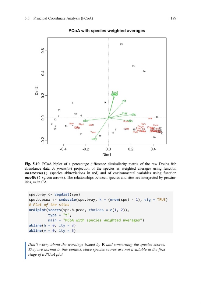
Fig. 5.10 PCoA biplot of a percentage difference dissimilarity matrix of the raw Doubs fish
abundance data. A posteriori projection of the species as weighted averages using function
wascores() (species abbreviations in red) and of environmental variables using function
envfit() (green arrows). The relationships between species and sites are interpreted by proximities, as in CA
5.5 Principal Coordinate Analysis (PCoA)
189
spe.b.pcoa <- cmdscale(spe.bray, k = (nrow(spe) - 1), eig = TRUE)
# Plot of the sites
ordiplot(scores(spe.b.pcoa, choices = c(1, 2)),
type = "t",
main = "PCoA with species weighted averages")
abline(h = 0, lty = 3)
abline(v = 0, lty = 3)
Don’t worry about the warnings issued by R and concerning the species scores.
They are normal in this context, since species scores are not available at the first
stage of a PCoA plot.
-0.4
-0.2
0.0
0.2
0.4
-0.2
0.0
0.2
0.4
0.6
PCoA with species weighted averages
Dim1
Dim2
1
2
3
4
5
6
7
9
10
11
12
13
14
15
16
17
18
19
20 21 22
23
24
25
26
27
28
29
30
Cogo
Satr
Phph
Babl
Thth
Teso
Chna
Pato
Lele
Sqce
Baba Albi
Gogo
Eslu
Pefl
Rham
Legi
Scer
Cyca
Titi
Abbr Icme
Gyce
Ruru
Blbj
Alal
Anan
dfs
ele
dis
har
pho
nit
amm
oxy
bod
Fig. 5.10 PCoA biplot of a percentage difference dissimilarity matrix of the raw Doubs fish
abundance data. A posteriori projection of the species as weighted averages using function
wascores() (species abbreviations in red) and of environmental variables using function
envfit() (green arrows). The relationships between species and sites are interpreted by proximities, as in CA
5.5 Principal Coordinate Analysis (PCoA)
189