

fact that the missing value is close or not to the mean of the variable (which was the
case for pho but not bod).
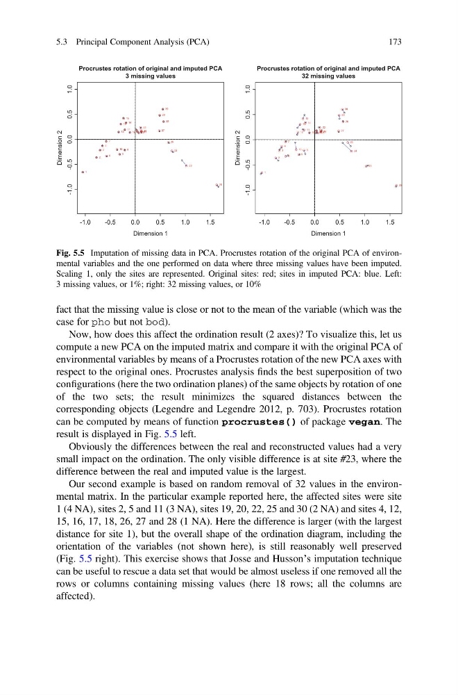
Now, how does this affect the ordination result (2 axes)? To visualize this, let us
compute a new PCA on the imputed matrix and compare it with the original PCA of
environmental variables by means of a Procrustes rotation of the new PCA axes with
respect to the original ones. Procrustes analysis finds the best superposition of two
configurations (here the two ordination planes) of the same objects by rotation of one
of the two sets; the result minimizes the squared distances between the
corresponding objects (Legendre and Legendre 2012, p. 703). Procrustes rotation
can be computed by means of function procrustes() of package vegan. The
result is displayed in Fig. 5.5 left.
Obviously the differences between the real and reconstructed values had a very
small impact on the ordination. The only visible difference is at site #23, where the
difference between the real and imputed value is the largest.
Our second example is based on random removal of 32 values in the environmental matrix. In the particular example reported here, the affected sites were site
1 (4 NA), sites 2, 5 and 11 (3 NA), sites 19, 20, 22, 25 and 30 (2 NA) and sites 4, 12,
15, 16, 17, 18, 26, 27 and 28 (1 NA). Here the difference is larger (with the largest
distance for site 1), but the overall shape of the ordination diagram, including the
orientation of the variables (not shown here), is still reasonably well preserved
(Fig. 5.5 right). This exercise shows that Josse and Husson’s imputation technique
can be useful to rescue a data set that would be almost useless if one removed all the
rows or columns containing missing values (here 18 rows; all the columns are
affected).
-1.0
-0.5
0.0
0.5
1.0
1.5
-1.0
-0.5
0.0
0.5
1.0
Procrustes rotation of original and imputed PCA
3 missing values
Dimension 1
Dimension 2
1
2
3
4
5
6
7
9
10
11
12
13 14
15
16
17
18
19 20
21
22
23
24
25
26
27
28
29
30
-1.0
-0.5
0.0
0.5
1.0
1.5
-1.0
-0.5
0.0
0.5
1.0
Procrustes rotation of original and imputed PCA
32 missing values
Dimension 1
Dimension 2
1
2
3
4
5
6
7
9
10
11
12
13 14
15
16
17
18
19 20
21
22
23
24
25
26
27
28
29
30
Fig. 5.5 Imputation of missing data in PCA. Procrustes rotation of the original PCA of environmental variables and the one performed on data where three missing values have been imputed.
Scaling 1, only the sites are represented. Original sites: red; sites in imputed PCA: blue. Left:
3 missing values, or 1%; right: 32 missing values, or 10%
5.3 Principal Component Analysis (PCA)
173
case for pho but not bod).
Now, how does this affect the ordination result (2 axes)? To visualize this, let us
compute a new PCA on the imputed matrix and compare it with the original PCA of
environmental variables by means of a Procrustes rotation of the new PCA axes with
respect to the original ones. Procrustes analysis finds the best superposition of two
configurations (here the two ordination planes) of the same objects by rotation of one
of the two sets; the result minimizes the squared distances between the
corresponding objects (Legendre and Legendre 2012, p. 703). Procrustes rotation
can be computed by means of function procrustes() of package vegan. The
result is displayed in Fig. 5.5 left.
Obviously the differences between the real and reconstructed values had a very
small impact on the ordination. The only visible difference is at site #23, where the
difference between the real and imputed value is the largest.
Our second example is based on random removal of 32 values in the environmental matrix. In the particular example reported here, the affected sites were site
1 (4 NA), sites 2, 5 and 11 (3 NA), sites 19, 20, 22, 25 and 30 (2 NA) and sites 4, 12,
15, 16, 17, 18, 26, 27 and 28 (1 NA). Here the difference is larger (with the largest
distance for site 1), but the overall shape of the ordination diagram, including the
orientation of the variables (not shown here), is still reasonably well preserved
(Fig. 5.5 right). This exercise shows that Josse and Husson’s imputation technique
can be useful to rescue a data set that would be almost useless if one removed all the
rows or columns containing missing values (here 18 rows; all the columns are
affected).
-1.0
-0.5
0.0
0.5
1.0
1.5
-1.0
-0.5
0.0
0.5
1.0
Procrustes rotation of original and imputed PCA
3 missing values
Dimension 1
Dimension 2
1
2
3
4
5
6
7
9
10
11
12
13 14
15
16
17
18
19 20
21
22
23
24
25
26
27
28
29
30
-1.0
-0.5
0.0
0.5
1.0
1.5
-1.0
-0.5
0.0
0.5
1.0
Procrustes rotation of original and imputed PCA
32 missing values
Dimension 1
Dimension 2
1
2
3
4
5
6
7
9
10
11
12
13 14
15
16
17
18
19 20
21
22
23
24
25
26
27
28
29
30
Fig. 5.5 Imputation of missing data in PCA. Procrustes rotation of the original PCA of environmental variables and the one performed on data where three missing values have been imputed.
Scaling 1, only the sites are represented. Original sites: red; sites in imputed PCA: blue. Left:
3 missing values, or 1%; right: 32 missing values, or 10%
5.3 Principal Component Analysis (PCA)
173