

# PCA of the environmental variables minus oxy and bod
env.pca2 <- rda(env[, -c(10, 11)], scale = TRUE)
# Create data frame with oxy and bod (our "new" variables)
new.var <- env[, c(10, 11)]
# Compute position of new variables (arrow tips)
new.vscores
newdata = new.var,
scaling = 2)
# Plot of the result - scaling 2
biplot(env.pca2, scaling = 2)
arrows(
0,
0,
new.vscores[, 1],
new.vscores[, 2],
length = 0.05,
angle = 30,
col = "blue"
)
text(
new.vscores[, 1],
new.vscores[, 2],
labels = rownames(new.vscores),
cex = 0.8,
col = "blue",
pos = 2
)
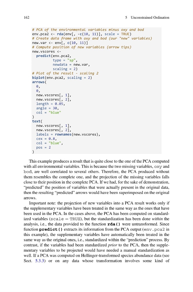
This example produces a result that is quite close to the one of the PCA computed
with all environmental variables. This is because the two missing variables, oxy and
bod, are well correlated to several others. Therefore, the PCA produced without
them resembles the complete one, and the projection of the missing variables falls
close to their position in the complete PCA. If we had, for the sake of demonstration,
“predicted” the position of variables that were actually present in the original data,
then the resulting “predicted” arrows would have been superimposed on the original
arrows.
Important note: the projection of new variables into a PCA result works only if
the supplementary variables have been treated in the same way as the ones that have
been used in the PCA. In the cases above, the PCA has been computed on standardized variables (scale ¼ TRUE), but the standardization has been done within the
analysis, i.e., the data provided to the function rda() were untransformed. Since
function predict() extracts its information from the PCA output (env.pca2 in
this example), the supplementary variables have automatically been treated in the
same way as the original ones, i.e., standardized within the “prediction” process. By
contrast, if the variables had been standardized prior to the PCA, then the supplementary variables to be projected would have needed a manual standardization as
well. If a PCA was computed on Hellinger-transformed species abundance data (see
Sect. 5.3.3) or on any data whose transformation involves some kind of
162
5 Unconstrained Ordination
env.pca2 <- rda(env[, -c(10, 11)], scale = TRUE)
# Create data frame with oxy and bod (our "new" variables)
new.var <- env[, c(10, 11)]
# Compute position of new variables (arrow tips)
new.vscores
newdata = new.var,
scaling = 2)
# Plot of the result - scaling 2
biplot(env.pca2, scaling = 2)
arrows(
0,
0,
new.vscores[, 1],
new.vscores[, 2],
length = 0.05,
angle = 30,
col = "blue"
)
text(
new.vscores[, 1],
new.vscores[, 2],
labels = rownames(new.vscores),
cex = 0.8,
col = "blue",
pos = 2
)
This example produces a result that is quite close to the one of the PCA computed
with all environmental variables. This is because the two missing variables, oxy and
bod, are well correlated to several others. Therefore, the PCA produced without
them resembles the complete one, and the projection of the missing variables falls
close to their position in the complete PCA. If we had, for the sake of demonstration,
“predicted” the position of variables that were actually present in the original data,
then the resulting “predicted” arrows would have been superimposed on the original
arrows.
Important note: the projection of new variables into a PCA result works only if
the supplementary variables have been treated in the same way as the ones that have
been used in the PCA. In the cases above, the PCA has been computed on standardized variables (scale ¼ TRUE), but the standardization has been done within the
analysis, i.e., the data provided to the function rda() were untransformed. Since
function predict() extracts its information from the PCA output (env.pca2 in
this example), the supplementary variables have automatically been treated in the
same way as the original ones, i.e., standardized within the “prediction” process. By
contrast, if the variables had been standardized prior to the PCA, then the supplementary variables to be projected would have needed a manual standardization as
well. If a PCA was computed on Hellinger-transformed species abundance data (see
Sect. 5.3.3) or on any data whose transformation involves some kind of
162
5 Unconstrained Ordination