

In a PCA ordination diagram, following the tradition of scatter diagrams in
Cartesian coordinate systems, objects are represented as points and variables are
displayed as arrows.
Later in this chapter (Sect. 5.7), you will see how to program a PCA in R using
matrix equations. But for everyday users, PCA is available in several R packages. A
convenient function for ecologists is rda() in package vegan. The name of the
function refers to redundancy analysis, a method that will be presented in Chap. 6.
Other possible functions are PCA.newr() provided with this book, or else dudi.
pca() (package ade4) and prcomp() (package stats).
5.3.2 PCA of the Environmental Variables of the Doubs River
Data Using rda()
Let us work again with the Doubs data. We have 11 quantitative environmental
variables at our disposal. How are they correlated? What can we learn from the
ordination of the sites?
Since the variables are expressed in different measurement scales (they are
dimensionally heterogeneous), we shall compute PCA from a correlation matrix.
Correlations are the covariances of standardized variables.
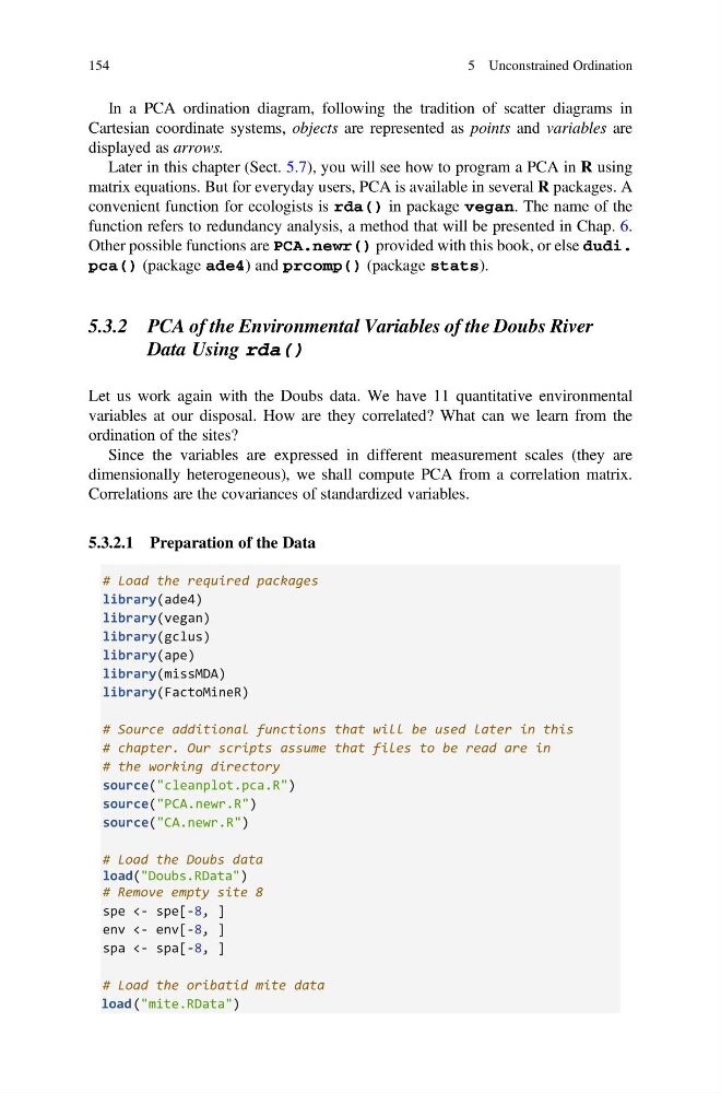
5.3.2.1 Preparation of the Data
library(ade4)
library(vegan)
library(gclus)
library(ape)
library(missMDA)
library(FactoMineR)
# Source additional functions that will be used later in this
# chapter. Our scripts assume that files to be read are in
# the working directory
source("cleanplot.pca.R")
source("PCA.newr.R")
source("CA.newr.R")
# Load the required packages
# Load the Doubs data
load
load
("Doubs.RData")
# Remove empty site 8
spe <- spe[-8, ]
env <- env[-8, ]
spa <- spa[-8, ]
("mite.RData")
# Load the oribatid mite data
154
5 Unconstrained Ordination
Cartesian coordinate systems, objects are represented as points and variables are
displayed as arrows.
Later in this chapter (Sect. 5.7), you will see how to program a PCA in R using
matrix equations. But for everyday users, PCA is available in several R packages. A
convenient function for ecologists is rda() in package vegan. The name of the
function refers to redundancy analysis, a method that will be presented in Chap. 6.
Other possible functions are PCA.newr() provided with this book, or else dudi.
pca() (package ade4) and prcomp() (package stats).
5.3.2 PCA of the Environmental Variables of the Doubs River
Data Using rda()
Let us work again with the Doubs data. We have 11 quantitative environmental
variables at our disposal. How are they correlated? What can we learn from the
ordination of the sites?
Since the variables are expressed in different measurement scales (they are
dimensionally heterogeneous), we shall compute PCA from a correlation matrix.
Correlations are the covariances of standardized variables.
5.3.2.1 Preparation of the Data
library(ade4)
library(vegan)
library(gclus)
library(ape)
library(missMDA)
library(FactoMineR)
# Source additional functions that will be used later in this
# chapter. Our scripts assume that files to be read are in
# the working directory
source("cleanplot.pca.R")
source("PCA.newr.R")
source("CA.newr.R")
# Load the required packages
# Load the Doubs data
load
load
("Doubs.RData")
# Remove empty site 8
spe <- spe[-8, ]
env <- env[-8, ]
spa <- spa[-8, ]
("mite.RData")
# Load the oribatid mite data
154
5 Unconstrained Ordination