

# Defuzzified site plot
plot(
dc.pcoa,
xlab = "MDS1",
ylab = "MDS2",
pch = clNum,
col = clNum
)
legend(
"topleft",
col = 1:(k + 1),
pch = 1:(k + 1),
legend = levels(as.factor(spefuz.g)),
bty = "n"
)
Finally, let us plot the fuzzy clusters on the map of the river (Fig. 4.40).
-0.6
-0.4
-0.2
0.0
0.2
0.4
0.6
-0.6
-0.4
-0.2
0.0
0.2
0.4
MDS1
MDS2
M1
M2
M3
M4
N
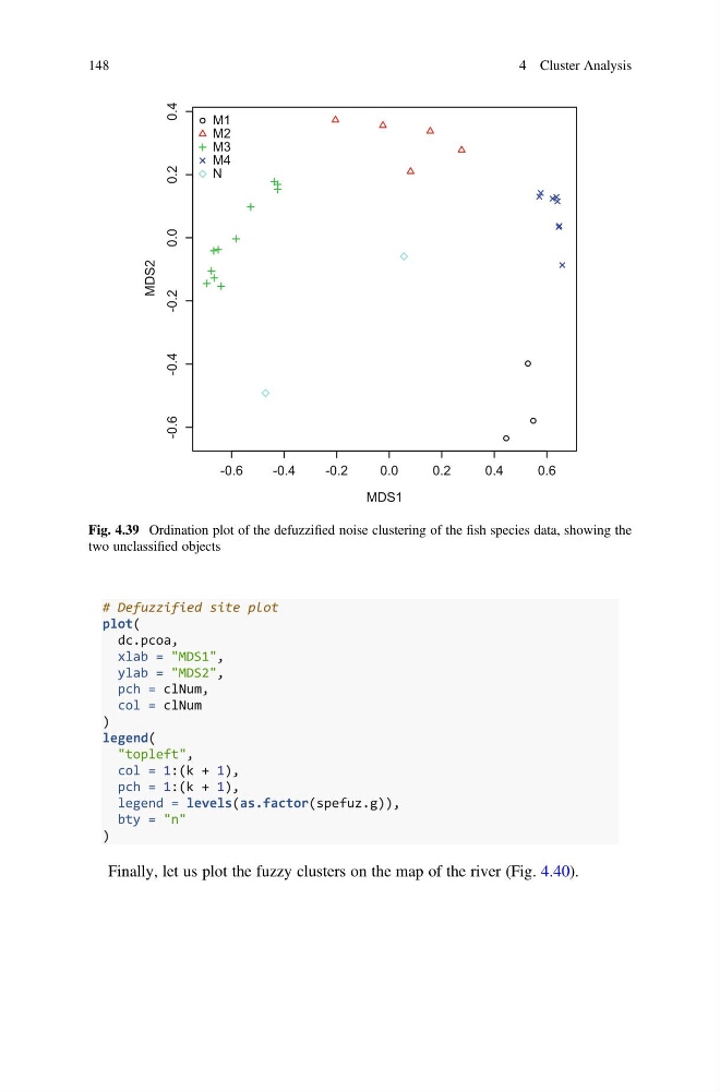
Fig. 4.39 Ordination plot of the defuzzified noise clustering of the fish species data, showing the
two unclassified objects
148
4 Cluster Analysis
plot(
dc.pcoa,
xlab = "MDS1",
ylab = "MDS2",
pch = clNum,
col = clNum
)
legend(
"topleft",
col = 1:(k + 1),
pch = 1:(k + 1),
legend = levels(as.factor(spefuz.g)),
bty = "n"
)
Finally, let us plot the fuzzy clusters on the map of the river (Fig. 4.40).
-0.6
-0.4
-0.2
0.0
0.2
0.4
0.6
-0.6
-0.4
-0.2
0.0
0.2
0.4
MDS1
MDS2
M1
M2
M3
M4
N
Fig. 4.39 Ordination plot of the defuzzified noise clustering of the fish species data, showing the
two unclassified objects
148
4 Cluster Analysis