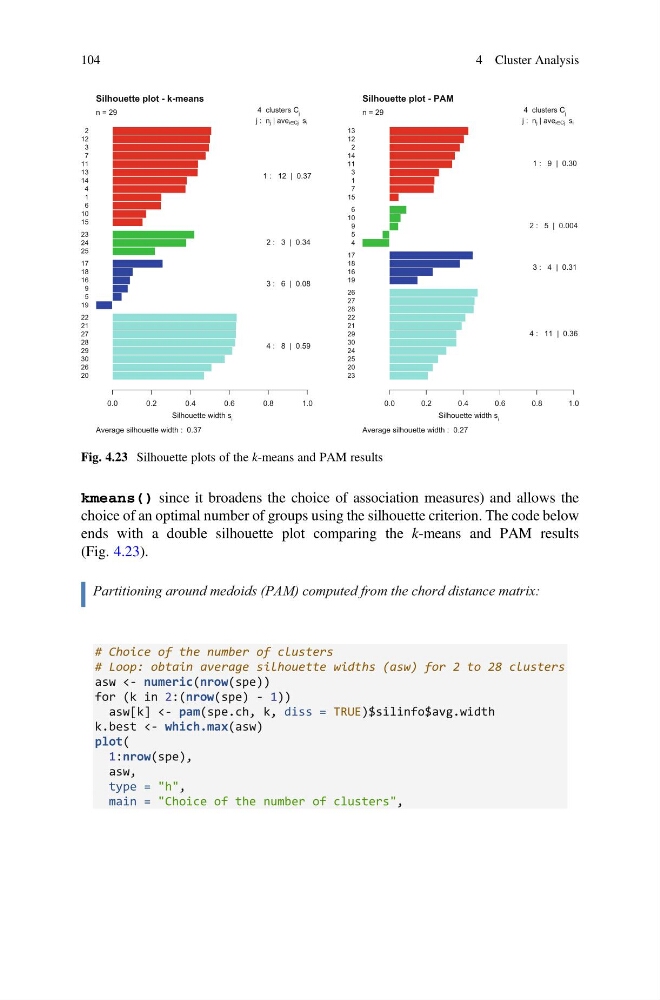
kmeans() since it broadens the choice of association measures) and allows the
choice of an optimal number of groups using the silhouette criterion. The code below
ends with a double silhouette plot comparing the k-means and PAM results
(Fig. 4.23).
Partitioning around medoids (PAM) computed from the chord distance matrix:
# Choice of the number of clusters
# Loop: obtain average silhouette widths (asw) for 2 to 28 clusters
asw <- numeric(nrow(spe))
for (k in 2:(nrow(spe) - 1))
asw[k] <- pam(spe.ch, k, diss = TRUE)$silinfo$avg.width
k.best <- which.max(asw)
plot(
1:nrow(spe),
asw,
type = "h",
main = "Choice of the number of clusters",
20
26
30
29
28
27
21
22
19
5
9
16
18
17
25
24
23
15
10
6
1
4
14
13
11
7
3
12
2
Silhouette width s i
0.0
0.2
0.4
0.6
0.8
1.0
Silhouette plot - k-means
Average silhouette width : 0.37
n = 29
j : nj | avei Cj si
1 : 12 | 0.37
2 : 3 | 0.34
3 : 6 | 0.08
4 : 8 | 0.59
23
20
25
24
30
29
21
22
28
27
26
19
16
18
17
4
5
9
10
6
15
7
1
3
11
14
2
12
13
Silhouette width s i
0.0
0.2
0.4
0.6
0.8
1.0
Silhouette plot - PAM
Average silhouette width : 0.27
n = 29
4 clusters C j
4 clusters C j
j : nj | avei Cj si
1 : 9 | 0.30
2 : 5 | 0.004
3 : 4 | 0.31
4 : 11 | 0.36
Fig. 4.23 Silhouette plots of the k-means and PAM results
104
4 Cluster Analysis