

23. Large-Scale Water Manipulations
treatment data should encompass periods of maximum and minimum soil water levels. Pretreatment
data for other variables that might logically trend
across a large experimental area (e.g., soil temperature) would also be useful.
An example of the use of pretreatment information as a base from which to judge the effectiveness
of a large-scale TDE is provided by Hanson et al.
(1998). They collected pretreatment measurements
of soil water content by TDR at an 8 X 8 m grid
across their experimental site (310 locations) from
April 1992 through July 12, 1993, and they found
significant pretreatment gradients in water content
across their experimental area driven by slope position and soil coarse fraction. From these pretreatment observations a covariate matrix was developed based on an individual measurement's
location according to the following equations:
Yij
Y
~ (Yijk)/n
~ (Yij)/n
(23.2)
(23.3)
347
CovYij = (Yij - Y)/sdY
(23.4)
where Yij is the mean annual value for a given location, Y is the grand mean for all locations and
times, i and j are the horizontal and vertical coordinates of the experimental area, k is the month of
the observation, and n is the number of observations for a given summation. As an illustration of
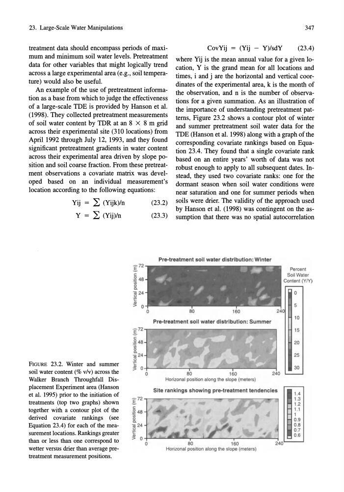
the importance of understanding pretreatment patterns, Figure 23.2 shows a contour plot of winter
and summer pretreatment soil water data for the
TDE (Hanson et al. 1998) along with a graph of the
corresponding covariate rankings based on Equation 23.4. They found that a single covariate rank
based on an entire years' worth of data was not
robust enough to apply to all subsequent dates. Instead, they used two covariate ranks: one for the
dormant season when soil water conditions were
near saturation and one for summer periods when
soils were drier. The validity of the approach used
by Hanson et al. (1998) was contingent on the assumption that there was no spatial autocorrelation
Pre.treatment soli water distribution: Winter
FIGURE 23.2. Winter and summer
soil water content (% v/v) across the
Walker Branch Throughfall Displacement Experiment area (Hanson
et al. 1995) prior to the initiation of
treatments (top two graphs) shown
together with a contour plot of the
derived covariate rankings (see
Equation 23.4) for each of the measurement locations. Rankings greater
than or less than one correspond to
wetter versus drier than average pretreatment measurement positions.
. :
I
•
I
;
. -
*..
#~
6./
t
.... '
.- f ~ ,
• . -II'~~
Percent
Soil Water
Content (YfY)
• o
5
:.
. .
. .
Pre-treatment soli water distribution: Summer
80
160
240
Horizonal position along the slope (meters)
Site rankings showing pre.treatment tendencies
80
160
240
Horizonal position along the slope (meters)
10
15
20
25
30
1.4
1.3
1.2
1.1
1
0.9
0.8
0.7
0.6
treatment data should encompass periods of maximum and minimum soil water levels. Pretreatment
data for other variables that might logically trend
across a large experimental area (e.g., soil temperature) would also be useful.
An example of the use of pretreatment information as a base from which to judge the effectiveness
of a large-scale TDE is provided by Hanson et al.
(1998). They collected pretreatment measurements
of soil water content by TDR at an 8 X 8 m grid
across their experimental site (310 locations) from
April 1992 through July 12, 1993, and they found
significant pretreatment gradients in water content
across their experimental area driven by slope position and soil coarse fraction. From these pretreatment observations a covariate matrix was developed based on an individual measurement's
location according to the following equations:
Yij
Y
~ (Yijk)/n
~ (Yij)/n
(23.2)
(23.3)
347
CovYij = (Yij - Y)/sdY
(23.4)
where Yij is the mean annual value for a given location, Y is the grand mean for all locations and
times, i and j are the horizontal and vertical coordinates of the experimental area, k is the month of
the observation, and n is the number of observations for a given summation. As an illustration of
the importance of understanding pretreatment patterns, Figure 23.2 shows a contour plot of winter
and summer pretreatment soil water data for the
TDE (Hanson et al. 1998) along with a graph of the
corresponding covariate rankings based on Equation 23.4. They found that a single covariate rank
based on an entire years' worth of data was not
robust enough to apply to all subsequent dates. Instead, they used two covariate ranks: one for the
dormant season when soil water conditions were
near saturation and one for summer periods when
soils were drier. The validity of the approach used
by Hanson et al. (1998) was contingent on the assumption that there was no spatial autocorrelation
Pre.treatment soli water distribution: Winter
FIGURE 23.2. Winter and summer
soil water content (% v/v) across the
Walker Branch Throughfall Displacement Experiment area (Hanson
et al. 1995) prior to the initiation of
treatments (top two graphs) shown
together with a contour plot of the
derived covariate rankings (see
Equation 23.4) for each of the measurement locations. Rankings greater
than or less than one correspond to
wetter versus drier than average pretreatment measurement positions.
. :
I
•
I
;
. -
*..
#~
6./
t
.... '
.- f ~ ,
• . -II'~~
Percent
Soil Water
Content (YfY)
• o
5
:.
. .
. .
Pre-treatment soli water distribution: Summer
80
160
240
Horizonal position along the slope (meters)
Site rankings showing pre.treatment tendencies
80
160
240
Horizonal position along the slope (meters)
10
15
20
25
30
1.4
1.3
1.2
1.1
1
0.9
0.8
0.7
0.6