

168
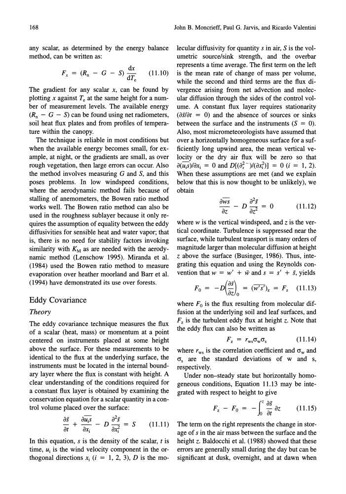
any scalar, as determined by the energy balance
method, can be written as:
dx
S) dT e
(11.10)
The gradient for any scalar x, can be found by
plotting x against Te at the same height for a number of measurement levels. The available energy
(Rn - G - S) can be found using net radiometers,
soil heat flux plates and from profiles of temperature within the canopy.
The technique is reliable in most conditions but
when the available energy becomes small, for example, at night, or the gradients are small, as over
rough vegetation, then large errors can occur. Also
the method involves measuring G and S, and this
poses problems. In low windspeed conditions,
where the aerodynamic method fails because of
stalling of anemometers, the Bowen ratio method
works well. The Bowen ratio method can also be
used in the roughness sub layer because it only requires the assumption of equality between the eddy
diffusivities for sensible heat and water vapor; that
is, there is no need for stability factors invoking
similarity with KM as are needed with the aerodynamic method (Lenschow 1995). Miranda et al.
(1984) used the Bowen ratio method to measure
evaporation over heather moorland and Barr et al.
(1994) have demonstrated its use over forests.
Eddy Covariance
Theory
The eddy covariance technique measures the flux
of a scalar (heat, mass) or momentum at a point
centered on instruments placed at some height
above the surface. For these measurements to be
identical to the flux at the underlying surface, the
instruments must be located in the internal boundary layer where the flux is constant with height. A
clear understanding of the conditions required for
a constant flux layer is obtained by examining the
conservation equation for a scalar quantity in a control volume placed over the surface:
(11.11)
In this equation, s is the density of the scalar, t is
time, Ui is the wind velocity component in the orthogonal directions Xi (i = 1, 2, 3), D is the moJohn B. Moncrieff, Paul G. Jarvis, and Ricardo Valentini
lecular diffusivity for quantity s in air, S is the volumetric source/sink strength, and the overbar
represents a time average. The first term on the left
is the mean rate of change of mass per volume,
while the second and third terms are the flux divergence arising from net advection and molecular diffusion through the sides of the control volume. A constant flux layer requires stationarity
(as/at = 0) and the absence of sources or sinks
between the surface and the instruments (S = 0).
Also, most micrometeorologists have assumed that
over a horizontally homogeneous surface for a sufficiently long upwind area, the mean vertical velocity or the dry air flux will be zero so that
a(UiS)/aXi = 0 and D[(a;-)l(axf)] = 0 (i = 1, 2).
When these assumptions are met (and we explain
below that this is now thought to be unlikely), we
obtain
aws
az
a 2 s
D - = 0
ar
(11.12)
where w is the vertical windspeed, and z is the vertical coordinate. Turbulence is suppressed near the
surface, while turbulent transport is many orders of
magnitude larger than molecular diffusion at height
z above the surface (Businger, 1986). Thus, integrating this equation and using the Reynolds convention that w = Wi + w and s = S' + s, yields
( as) ----, I
11 3
Fo = - D az 0 = (w s)z = Fz ( .1)
where Fo is the flux resulting from molecular diffusion at the underlying soil and leaf surfaces, and
Fz is the turbulent eddy flux at height z. Note that
the eddy flux can also be written as
(11.14)
where rws is the correlation coefficient and o"w and
o"s are the standard deviations of w and s,
respectively.
Under non-steady state but horizontally homogeneous conditions, Equation 11.13 may be integrated with respect to height to give
i
z as
F - Fo = -
- az
z
0 at
(11.15)
The term on the right represents the change in storage of s in the air mass between the surface and the
height z. Baldocchi et al. (1988) showed that these
errors are generally small during the day but can be
significant at dusk, overnight, and at dawn when
any scalar, as determined by the energy balance
method, can be written as:
dx
S) dT e
(11.10)
The gradient for any scalar x, can be found by
plotting x against Te at the same height for a number of measurement levels. The available energy
(Rn - G - S) can be found using net radiometers,
soil heat flux plates and from profiles of temperature within the canopy.
The technique is reliable in most conditions but
when the available energy becomes small, for example, at night, or the gradients are small, as over
rough vegetation, then large errors can occur. Also
the method involves measuring G and S, and this
poses problems. In low windspeed conditions,
where the aerodynamic method fails because of
stalling of anemometers, the Bowen ratio method
works well. The Bowen ratio method can also be
used in the roughness sub layer because it only requires the assumption of equality between the eddy
diffusivities for sensible heat and water vapor; that
is, there is no need for stability factors invoking
similarity with KM as are needed with the aerodynamic method (Lenschow 1995). Miranda et al.
(1984) used the Bowen ratio method to measure
evaporation over heather moorland and Barr et al.
(1994) have demonstrated its use over forests.
Eddy Covariance
Theory
The eddy covariance technique measures the flux
of a scalar (heat, mass) or momentum at a point
centered on instruments placed at some height
above the surface. For these measurements to be
identical to the flux at the underlying surface, the
instruments must be located in the internal boundary layer where the flux is constant with height. A
clear understanding of the conditions required for
a constant flux layer is obtained by examining the
conservation equation for a scalar quantity in a control volume placed over the surface:
(11.11)
In this equation, s is the density of the scalar, t is
time, Ui is the wind velocity component in the orthogonal directions Xi (i = 1, 2, 3), D is the moJohn B. Moncrieff, Paul G. Jarvis, and Ricardo Valentini
lecular diffusivity for quantity s in air, S is the volumetric source/sink strength, and the overbar
represents a time average. The first term on the left
is the mean rate of change of mass per volume,
while the second and third terms are the flux divergence arising from net advection and molecular diffusion through the sides of the control volume. A constant flux layer requires stationarity
(as/at = 0) and the absence of sources or sinks
between the surface and the instruments (S = 0).
Also, most micrometeorologists have assumed that
over a horizontally homogeneous surface for a sufficiently long upwind area, the mean vertical velocity or the dry air flux will be zero so that
a(UiS)/aXi = 0 and D[(a;-)l(axf)] = 0 (i = 1, 2).
When these assumptions are met (and we explain
below that this is now thought to be unlikely), we
obtain
aws
az
a 2 s
D - = 0
ar
(11.12)
where w is the vertical windspeed, and z is the vertical coordinate. Turbulence is suppressed near the
surface, while turbulent transport is many orders of
magnitude larger than molecular diffusion at height
z above the surface (Businger, 1986). Thus, integrating this equation and using the Reynolds convention that w = Wi + w and s = S' + s, yields
( as) ----, I
11 3
Fo = - D az 0 = (w s)z = Fz ( .1)
where Fo is the flux resulting from molecular diffusion at the underlying soil and leaf surfaces, and
Fz is the turbulent eddy flux at height z. Note that
the eddy flux can also be written as
(11.14)
where rws is the correlation coefficient and o"w and
o"s are the standard deviations of w and s,
respectively.
Under non-steady state but horizontally homogeneous conditions, Equation 11.13 may be integrated with respect to height to give
i
z as
F - Fo = -
- az
z
0 at
(11.15)
The term on the right represents the change in storage of s in the air mass between the surface and the
height z. Baldocchi et al. (1988) showed that these
errors are generally small during the day but can be
significant at dusk, overnight, and at dawn when