

8.4 TOPOGRlD
221
(a) Lanice and Mytilus
(c) Lanice
(b) Classification after Hertweck
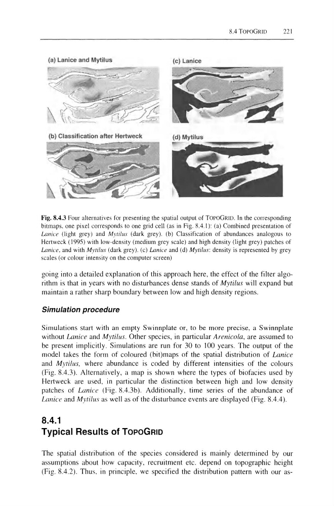
Fig. 8.4.3 Four alternatives for presenting the spatial output of TOPOGRID. In the corresponding
bitmaps, one pixel corresponds to one grid cell (as in Fig. 8.4.1): (a) Combined presentation of
ulI1iee (light grey) and Myri/us (dark grey). (b) Classification of abundances analogous to
Hertweck (1995) with low-density (medium grey scale) and high density (light grey) patches of
Laniee, and with Mytilus (dark grey). (e) umice and (d) Mytilus: density is represented by grey
scales (or colour intensity on the computer screen)
going into a detailed explanation of this approach here, the effect of the filter algorithm is that in years with no disturbances dense stands of Mytilus will expand but
maintain a rather sharp boundary between low and high density regions.
Simulation procedure
Simulations start with an empty Swinnplate or, to be more precise, a Swinnplate
without Lanice and Mytilus. Other species, in particular Arenicola, are assumed to
be present implicitly. Simulations are run for 30 to 100 years. The output of the
model takes the form of coloured (bit)maps of the spatial distribution of Lanice
and Mytilus, where abundance is coded by different intensities of the colours
(Fig. 8.4.3). Alternatively, a map is shown where the types of biofacies used by
Hertweck are used, in particular the distinction between high and low density
patches of Lanice (Fig.8.4.3b). Additionally, time series of the abundance of
Lanice and Mytilus as well as of the disturbance events are displayed (Fig. 8.4.4).
8.4.1
Typical Results of TOPOGRID
The spatial distribution of the species considered is mainly determined by our
assumptions about how capacity, recruitment etc. depend on topographic height
(Fig. 8.4.2). Thus. in principle, we specified the distribution pattern with our as-
221
(a) Lanice and Mytilus
(c) Lanice
(b) Classification after Hertweck
Fig. 8.4.3 Four alternatives for presenting the spatial output of TOPOGRID. In the corresponding
bitmaps, one pixel corresponds to one grid cell (as in Fig. 8.4.1): (a) Combined presentation of
ulI1iee (light grey) and Myri/us (dark grey). (b) Classification of abundances analogous to
Hertweck (1995) with low-density (medium grey scale) and high density (light grey) patches of
Laniee, and with Mytilus (dark grey). (e) umice and (d) Mytilus: density is represented by grey
scales (or colour intensity on the computer screen)
going into a detailed explanation of this approach here, the effect of the filter algorithm is that in years with no disturbances dense stands of Mytilus will expand but
maintain a rather sharp boundary between low and high density regions.
Simulation procedure
Simulations start with an empty Swinnplate or, to be more precise, a Swinnplate
without Lanice and Mytilus. Other species, in particular Arenicola, are assumed to
be present implicitly. Simulations are run for 30 to 100 years. The output of the
model takes the form of coloured (bit)maps of the spatial distribution of Lanice
and Mytilus, where abundance is coded by different intensities of the colours
(Fig. 8.4.3). Alternatively, a map is shown where the types of biofacies used by
Hertweck are used, in particular the distinction between high and low density
patches of Lanice (Fig.8.4.3b). Additionally, time series of the abundance of
Lanice and Mytilus as well as of the disturbance events are displayed (Fig. 8.4.4).
8.4.1
Typical Results of TOPOGRID
The spatial distribution of the species considered is mainly determined by our
assumptions about how capacity, recruitment etc. depend on topographic height
(Fig. 8.4.2). Thus. in principle, we specified the distribution pattern with our as-