

The drivers in this system are actually the concentration differences expressed in
the six flows. Here we assumed that all volumes are 1.0. Make each stock a different
volume. Even make one of them a function of time as in a collapsing balloon.
Then set up converters for the four stocks that represent their dynamic concentrations. (Remember, the stocks are measuring the weight such as in grams of gas in
each of them. The concentrations are then in grams per unit volume.) Have the
concentration differences times a specific diffusion constant for each flow be
the flow equation in each of the six cases. This is a more realistic representation
of diffusion conditions.
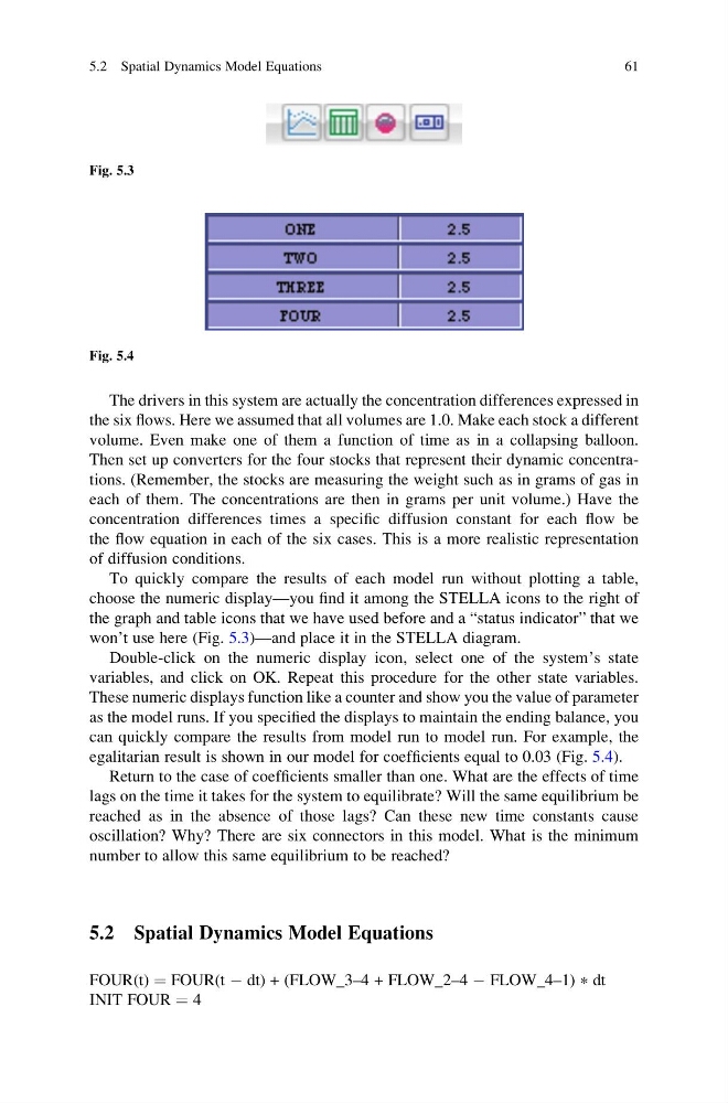
To quickly compare the results of each model run without plotting a table,
choose the numeric display—you find it among the STELLA icons to the right of
the graph and table icons that we have used before and a “status indicator” that we
won’t use here (Fig. 5.3)—and place it in the STELLA diagram.
Double-click on the numeric display icon, select one of the system’s state
variables, and click on OK. Repeat this procedure for the other state variables.
These numeric displays function like a counter and show you the value of parameter
as the model runs. If you specified the displays to maintain the ending balance, you
can quickly compare the results from model run to model run. For example, the
egalitarian result is shown in our model for coefficients equal to 0.03 (Fig. 5.4).
Return to the case of coefficients smaller than one. What are the effects of time
lags on the time it takes for the system to equilibrate? Will the same equilibrium be
reached as in the absence of those lags? Can these new time constants cause
oscillation? Why? There are six connectors in this model. What is the minimum
number to allow this same equilibrium to be reached?
5.2 Spatial Dynamics Model Equations
FOUR(t) ¼ FOUR(t À dt) + (FLOW_3–4 + FLOW_2–4 À FLOW_4–1) * dt
INIT FOUR ¼ 4
Fig. 5.3
Fig. 5.4
5.2 Spatial Dynamics Model Equations
61
the six flows. Here we assumed that all volumes are 1.0. Make each stock a different
volume. Even make one of them a function of time as in a collapsing balloon.
Then set up converters for the four stocks that represent their dynamic concentrations. (Remember, the stocks are measuring the weight such as in grams of gas in
each of them. The concentrations are then in grams per unit volume.) Have the
concentration differences times a specific diffusion constant for each flow be
the flow equation in each of the six cases. This is a more realistic representation
of diffusion conditions.
To quickly compare the results of each model run without plotting a table,
choose the numeric display—you find it among the STELLA icons to the right of
the graph and table icons that we have used before and a “status indicator” that we
won’t use here (Fig. 5.3)—and place it in the STELLA diagram.
Double-click on the numeric display icon, select one of the system’s state
variables, and click on OK. Repeat this procedure for the other state variables.
These numeric displays function like a counter and show you the value of parameter
as the model runs. If you specified the displays to maintain the ending balance, you
can quickly compare the results from model run to model run. For example, the
egalitarian result is shown in our model for coefficients equal to 0.03 (Fig. 5.4).
Return to the case of coefficients smaller than one. What are the effects of time
lags on the time it takes for the system to equilibrate? Will the same equilibrium be
reached as in the absence of those lags? Can these new time constants cause
oscillation? Why? There are six connectors in this model. What is the minimum
number to allow this same equilibrium to be reached?
5.2 Spatial Dynamics Model Equations
FOUR(t) ¼ FOUR(t À dt) + (FLOW_3–4 + FLOW_2–4 À FLOW_4–1) * dt
INIT FOUR ¼ 4
Fig. 5.3
Fig. 5.4
5.2 Spatial Dynamics Model Equations
61