

Such prediction is impossible. Run the model over and over again, and you will find
that always the same path is chosen. The system that we are dealing with here is not
random, it is deterministic. Yet, prediction from past and current states is impossible. Recognize also that if you change even very slightly the initial conditions, e.
g., N ¼ 0.101 instead of N ¼ 0.1, a very different path emerges. This should
illustrate the sensitivity of nonlinear dynamic systems to initial conditions, and
sensitize you to the limitations of real data—which always comes with measurement errors—in forecasting a system’s behavior.
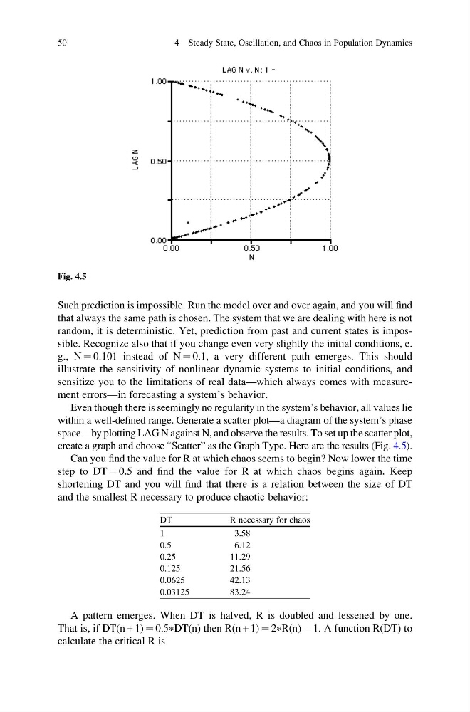
Even though there is seemingly no regularity in the system’s behavior, all values lie
within a well-defined range. Generate a scatter plot—a diagram of the system’s phase
space—by plotting LAG N against N, and observe the results. To set up the scatter plot,
create a graph and choose “Scatter” as the Graph Type. Here are the results (Fig. 4.5).
Can you find the value for R at which chaos seems to begin? Now lower the time
step to DT ¼ 0.5 and find the value for R at which chaos begins again. Keep
shortening DT and you will find that there is a relation between the size of DT
and the smallest R necessary to produce chaotic behavior:
DT
R necessary for chaos
1
3.58
0.5
6.12
0.25
11.29
0.125
21.56
0.0625
42.13
0.03125
83.24
A pattern emerges. When DT is halved, R is doubled and lessened by one.
That is, if DT(n + 1) ¼ 0.5 * DT(n) then R(n + 1) ¼ 2 * R(n) À 1. A function R(DT) to
calculate the critical R is
Fig. 4.5
50
4 Steady State, Oscillation, and Chaos in Population Dynamics
that always the same path is chosen. The system that we are dealing with here is not
random, it is deterministic. Yet, prediction from past and current states is impossible. Recognize also that if you change even very slightly the initial conditions, e.
g., N ¼ 0.101 instead of N ¼ 0.1, a very different path emerges. This should
illustrate the sensitivity of nonlinear dynamic systems to initial conditions, and
sensitize you to the limitations of real data—which always comes with measurement errors—in forecasting a system’s behavior.
Even though there is seemingly no regularity in the system’s behavior, all values lie
within a well-defined range. Generate a scatter plot—a diagram of the system’s phase
space—by plotting LAG N against N, and observe the results. To set up the scatter plot,
create a graph and choose “Scatter” as the Graph Type. Here are the results (Fig. 4.5).
Can you find the value for R at which chaos seems to begin? Now lower the time
step to DT ¼ 0.5 and find the value for R at which chaos begins again. Keep
shortening DT and you will find that there is a relation between the size of DT
and the smallest R necessary to produce chaotic behavior:
DT
R necessary for chaos
1
3.58
0.5
6.12
0.25
11.29
0.125
21.56
0.0625
42.13
0.03125
83.24
A pattern emerges. When DT is halved, R is doubled and lessened by one.
That is, if DT(n + 1) ¼ 0.5 * DT(n) then R(n + 1) ¼ 2 * R(n) À 1. A function R(DT) to
calculate the critical R is
Fig. 4.5
50
4 Steady State, Oscillation, and Chaos in Population Dynamics