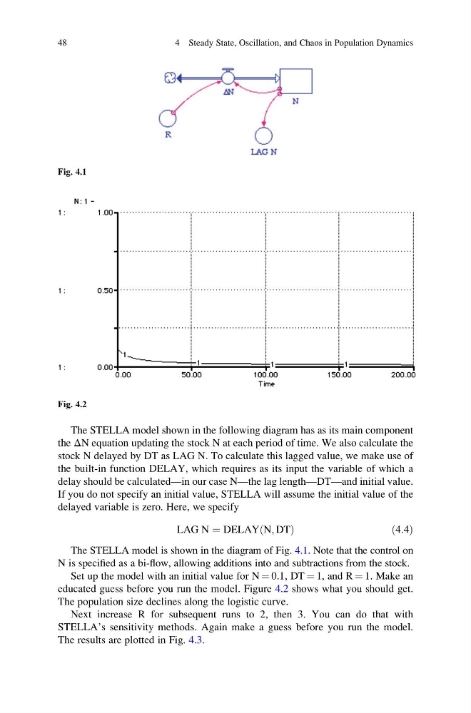
The STELLA model shown in the following diagram has as its main component
the ΔN equation updating the stock N at each period of time. We also calculate the
stock N delayed by DT as LAG N. To calculate this lagged value, we make use of
the built-in function DELAY, which requires as its input the variable of which a
delay should be calculated—in our case N—the lag length—DT—and initial value.
If you do not specify an initial value, STELLA will assume the initial value of the
delayed variable is zero. Here, we specify
LAG N ¼ DELAY N; DT
ð
Þ
ð4:4Þ
The STELLA model is shown in the diagram of Fig. 4.1. Note that the control on
N is specified as a bi-flow, allowing additions into and subtractions from the stock.
Set up the model with an initial value for N ¼ 0.1, DT ¼ 1, and R ¼ 1. Make an
educated guess before you run the model. Figure 4.2 shows what you should get.
The population size declines along the logistic curve.
Next increase R for subsequent runs to 2, then 3. You can do that with
STELLA’s sensitivity methods. Again make a guess before you run the model.
The results are plotted in Fig. 4.3.
Fig. 4.1
Fig. 4.2
48
4 Steady State, Oscillation, and Chaos in Population Dynamics