

5 years, that is, for convenience the stocking should occur about every 5 years.
Thus, to predict the full effect of the fish, a 10-year period is set as the modeling
time: fish are introduced in the spring of the first and the fifth year. Spring is chosen
to maximize the survival rate of the young fish. An area of 1,000 m
2 is chosen as the
basic unit of waterway area. The targeted water area is that portion of the waterway
up to 6 m in depth. The data used here are reported in Wiley et al. [1].
There are three basic parts to this model: the number of fish, the average size of
the fish, and the plant biomass. Let us first turn to the model component that deals
with the number of fish.
In the following figure, the input to the number of carp, which we here call
STOCK Rate, specifies when and how many 200 g fish are added to the waterway.
The output flows, which diminish the number of fish, are grouped under the control
MORTALITY. They are:
• PRED MORT, the consumption of the carp by the larger sport fish;
• WINTER MORT, the death of fish due to the harshness of the winter months;
and,
• STARVE MORT, the death of the carp due to lack of food.
Predator mortality is a function of the winter period, WINTER, a mortality
coefficient, MORT COEF, and the number of fish. The mortality coefficient, in
turn, is a function of the average age and size of the fish and a variable that causes
the mortality rate to increase as the fish ages, MORT COEF AGE. Winter mortality is
a function of the number of fish, the winter period, WINTER FLAG, and the above
aging coefficient. The WINTER FLAG indicates when winter occurs. It is defined as
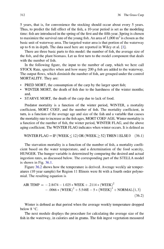
WINTER FLAG ¼ IF WEEK 12
ð
Þ OR WEEK ! 52
ð
Þ THEN 1 ELSE 0 ð36:1Þ
The starvation mortality is a function of the number of fish, a mortality coefficient based on the water temperature, and a determination of the food scarcity,
HUNGER. The hunger variable is determined by comparing the desired and actual
ingestion rates, as discussed below. The corresponding part of the STELLA model
is shown in Fig. 36.1.
Figure 36.2 shows how the temperature is derived. Average weekly air temperatures (10 year sample) for Region 11 Illinois were fit with a fourth order polynomial. The resulting equation is
AIR TEMP ¼ À 2:8474 À 1:025 Ã WEEK þ :2114 Ã WEEK
ð
Þ
2
À :0066 Ã WEEK
ð
Þ
3 þ 5:548E À 5 Ã
À
WEEK
Á 4 þ NORMAL
À
1, 3
Á
ð36:2Þ
Winter is defined as that period when the average weekly temperature dropped
below 8
C.
The next module displays the procedure for calculating the average size of the
fish in the waterway, in calories and in grams. The fish ingest vegetation measured
312
36 The Grass Carp
Thus, to predict the full effect of the fish, a 10-year period is set as the modeling
time: fish are introduced in the spring of the first and the fifth year. Spring is chosen
to maximize the survival rate of the young fish. An area of 1,000 m
2 is chosen as the
basic unit of waterway area. The targeted water area is that portion of the waterway
up to 6 m in depth. The data used here are reported in Wiley et al. [1].
There are three basic parts to this model: the number of fish, the average size of
the fish, and the plant biomass. Let us first turn to the model component that deals
with the number of fish.
In the following figure, the input to the number of carp, which we here call
STOCK Rate, specifies when and how many 200 g fish are added to the waterway.
The output flows, which diminish the number of fish, are grouped under the control
MORTALITY. They are:
• PRED MORT, the consumption of the carp by the larger sport fish;
• WINTER MORT, the death of fish due to the harshness of the winter months;
and,
• STARVE MORT, the death of the carp due to lack of food.
Predator mortality is a function of the winter period, WINTER, a mortality
coefficient, MORT COEF, and the number of fish. The mortality coefficient, in
turn, is a function of the average age and size of the fish and a variable that causes
the mortality rate to increase as the fish ages, MORT COEF AGE. Winter mortality is
a function of the number of fish, the winter period, WINTER FLAG, and the above
aging coefficient. The WINTER FLAG indicates when winter occurs. It is defined as
WINTER FLAG ¼ IF WEEK 12
ð
Þ OR WEEK ! 52
ð
Þ THEN 1 ELSE 0 ð36:1Þ
The starvation mortality is a function of the number of fish, a mortality coefficient based on the water temperature, and a determination of the food scarcity,
HUNGER. The hunger variable is determined by comparing the desired and actual
ingestion rates, as discussed below. The corresponding part of the STELLA model
is shown in Fig. 36.1.
Figure 36.2 shows how the temperature is derived. Average weekly air temperatures (10 year sample) for Region 11 Illinois were fit with a fourth order polynomial. The resulting equation is
AIR TEMP ¼ À 2:8474 À 1:025 Ã WEEK þ :2114 Ã WEEK
ð
Þ
2
À :0066 Ã WEEK
ð
Þ
3 þ 5:548E À 5 Ã
À
WEEK
Á 4 þ NORMAL
À
1, 3
Á
ð36:2Þ
Winter is defined as that period when the average weekly temperature dropped
below 8
C.
The next module displays the procedure for calculating the average size of the
fish in the waterway, in calories and in grams. The fish ingest vegetation measured
312
36 The Grass Carp