

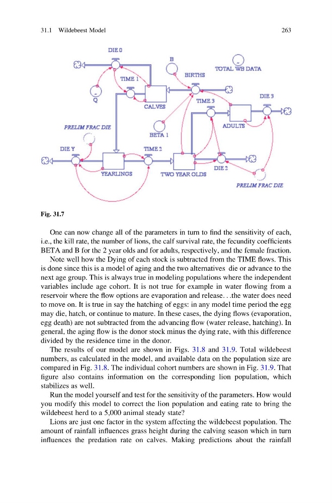
One can now change all of the parameters in turn to find the sensitivity of each,
i.e., the kill rate, the number of lions, the calf survival rate, the fecundity coefficients
BETA and B for the 2 year olds and for adults, respectively, and the female fraction.
Note well how the Dying of each stock is subtracted from the TIME flows. This
is done since this is a model of aging and the two alternatives die or advance to the
next age group. This is always true in modeling populations where the independent
variables include age cohort. It is not true for example in water flowing from a
reservoir where the flow options are evaporation and release. . .the water does need
to move on. It is true in say the hatching of eggs: in any model time period the egg
may die, hatch, or continue to mature. In these cases, the dying flows (evaporation,
egg death) are not subtracted from the advancing flow (water release, hatching). In
general, the aging flow is the donor stock minus the dying rate, with this difference
divided by the residence time in the donor.
The results of our model are shown in Figs. 31.8 and 31.9. Total wildebeest
numbers, as calculated in the model, and available data on the population size are
compared in Fig. 31.8. The individual cohort numbers are shown in Fig. 31.9. That
figure also contains information on the corresponding lion population, which
stabilizes as well.
Run the model yourself and test for the sensitivity of the parameters. How would
you modify this model to correct the lion population and eating rate to bring the
wildebeest herd to a 5,000 animal steady state?
Lions are just one factor in the system affecting the wildebeest population. The
amount of rainfall influences grass height during the calving season which in turn
influences the predation rate on calves. Making predictions about the rainfall
Fig. 31.7
31.1 Wildebeest Model
263
i.e., the kill rate, the number of lions, the calf survival rate, the fecundity coefficients
BETA and B for the 2 year olds and for adults, respectively, and the female fraction.
Note well how the Dying of each stock is subtracted from the TIME flows. This
is done since this is a model of aging and the two alternatives die or advance to the
next age group. This is always true in modeling populations where the independent
variables include age cohort. It is not true for example in water flowing from a
reservoir where the flow options are evaporation and release. . .the water does need
to move on. It is true in say the hatching of eggs: in any model time period the egg
may die, hatch, or continue to mature. In these cases, the dying flows (evaporation,
egg death) are not subtracted from the advancing flow (water release, hatching). In
general, the aging flow is the donor stock minus the dying rate, with this difference
divided by the residence time in the donor.
The results of our model are shown in Figs. 31.8 and 31.9. Total wildebeest
numbers, as calculated in the model, and available data on the population size are
compared in Fig. 31.8. The individual cohort numbers are shown in Fig. 31.9. That
figure also contains information on the corresponding lion population, which
stabilizes as well.
Run the model yourself and test for the sensitivity of the parameters. How would
you modify this model to correct the lion population and eating rate to bring the
wildebeest herd to a 5,000 animal steady state?
Lions are just one factor in the system affecting the wildebeest population. The
amount of rainfall influences grass height during the calving season which in turn
influences the predation rate on calves. Making predictions about the rainfall
Fig. 31.7
31.1 Wildebeest Model
263