

NEW WORM 2 ¼ IF LIFE 1 > 0 AND COIN 1 < :5
ð
Þ THEN LIFE 1 À 2
ELSE IF LIFE 1 > 0 AND COIN 1 > :5
ð
Þ THEN LIFE 1 þ 2
ELSE 0
ð13:11Þ
Now our model is finished. We have modules that we use to generate random pairs
of worms, to compare their lengths and let the longer one win a fight, and to generate
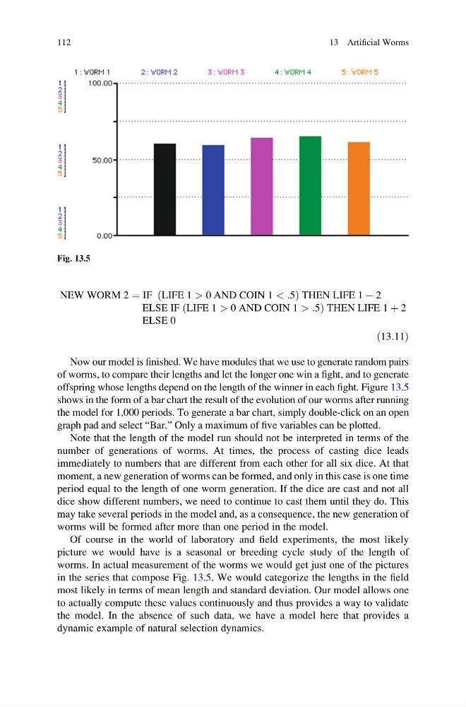
offspring whose lengths depend on the length of the winner in each fight. Figure 13.5
shows in the form of a bar chart the result of the evolution of our worms after running
the model for 1,000 periods. To generate a bar chart, simply double-click on an open
graph pad and select “Bar.” Only a maximum of five variables can be plotted.
Note that the length of the model run should not be interpreted in terms of the
number of generations of worms. At times, the process of casting dice leads
immediately to numbers that are different from each other for all six dice. At that
moment, a new generation of worms can be formed, and only in this case is one time
period equal to the length of one worm generation. If the dice are cast and not all
dice show different numbers, we need to continue to cast them until they do. This
may take several periods in the model and, as a consequence, the new generation of
worms will be formed after more than one period in the model.
Of course in the world of laboratory and field experiments, the most likely
picture we would have is a seasonal or breeding cycle study of the length of
worms. In actual measurement of the worms we would get just one of the pictures
in the series that compose Fig. 13.5. We would categorize the lengths in the field
most likely in terms of mean length and standard deviation. Our model allows one
to actually compute these values continuously and thus provides a way to validate
the model. In the absence of such data, we have a model here that provides a
dynamic example of natural selection dynamics.
Fig. 13.5
112
13 Artificial Worms
ð
Þ THEN LIFE 1 À 2
ELSE IF LIFE 1 > 0 AND COIN 1 > :5
ð
Þ THEN LIFE 1 þ 2
ELSE 0
ð13:11Þ
Now our model is finished. We have modules that we use to generate random pairs
of worms, to compare their lengths and let the longer one win a fight, and to generate
offspring whose lengths depend on the length of the winner in each fight. Figure 13.5
shows in the form of a bar chart the result of the evolution of our worms after running
the model for 1,000 periods. To generate a bar chart, simply double-click on an open
graph pad and select “Bar.” Only a maximum of five variables can be plotted.
Note that the length of the model run should not be interpreted in terms of the
number of generations of worms. At times, the process of casting dice leads
immediately to numbers that are different from each other for all six dice. At that
moment, a new generation of worms can be formed, and only in this case is one time
period equal to the length of one worm generation. If the dice are cast and not all
dice show different numbers, we need to continue to cast them until they do. This
may take several periods in the model and, as a consequence, the new generation of
worms will be formed after more than one period in the model.
Of course in the world of laboratory and field experiments, the most likely
picture we would have is a seasonal or breeding cycle study of the length of
worms. In actual measurement of the worms we would get just one of the pictures
in the series that compose Fig. 13.5. We would categorize the lengths in the field
most likely in terms of mean length and standard deviation. Our model allows one
to actually compute these values continuously and thus provides a way to validate
the model. In the absence of such data, we have a model here that provides a
dynamic example of natural selection dynamics.
Fig. 13.5
112
13 Artificial Worms