

5. Risk Assessment of a Proposed Introduction of Pacific Salmon
65
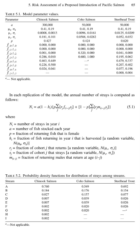
Table 5.1. Model parameter values.
Parameter
Chinook Salmon
Coho Salmon
Steelhead Trout
a
300,000
50,000
50,000
µ h , σ h
0.41, 0.19
0.41, 0.19
0.41, 0.19
µ r , σ r
0.0008, 0.0013
0.0096, 0.0161
0.0125, 0.0209
µ s , σ s
0.181, 0.101
0.0588, 0.0282
0.052, 0.032
p
0.427
0.424
0.620
f –,0 , f –,0
0.000, 0.000
0.000, 0.000
0.000, 0.000
f –,1 , f –,1
0.000, 0.000
0.000, 0.000
0.000, 0.000
f –,2 , f –,2
0.001, 0.000
0.320, 0.000
0.041, 0.000
f –,3 , f –,3
0.286, 0.010
0.680, 1.000
0.195, 0.062
f –,4 , f –,4
0.463, 0.449
— a
0.479, 0.337
f –,5 , f –,5
0.226, 0.500
—
0.207, 0.402
f –,6 , f –,6
0.024, 0.041
—
0.077, 0.196
f –,7 , f –,7
—
—
0.000, 0.004
a — Not applicable.
In each replication of the model, the annual number of strays is computed as
follows:
N i = a(1 − h i ){p͚
j
[r j f (i − j) s j ] + [1 − p]͚
j
[r j m (i − j) s j ]}
(5.1)
where
N i = number of strays in year i
a = number of fish stocked each year
p = fraction of returning fish that is female
h i = fraction of fish returning in year i that is harvested [a random variable,
N(µ h , σ h )]
r j = fraction of cohort j that returns [a random variable, N(µ r , σ r )]
s j = fraction of cohort j that strays [a random variable, N(µ s , σ s ])
m (i−j) = fraction of returning males that return at age (i−j)
Table 5.2. Probability density functions for distribution of strays among streams.
Stream
Chinook Salmon
Coho Salmon
Steelhead Trout
A
0.760
0.549
0.692
B
0.184
0.176
0.154
C
0.027
0.157
0.077
D
0.007
0.039
0.026
E
0.007
0.039
0.026
F
0.002
0.020
0.026
G
0.002
0.020
— a
H
0.002
—
—
I
0.002
—
—
a —Not applicable.
65
Table 5.1. Model parameter values.
Parameter
Chinook Salmon
Coho Salmon
Steelhead Trout
a
300,000
50,000
50,000
µ h , σ h
0.41, 0.19
0.41, 0.19
0.41, 0.19
µ r , σ r
0.0008, 0.0013
0.0096, 0.0161
0.0125, 0.0209
µ s , σ s
0.181, 0.101
0.0588, 0.0282
0.052, 0.032
p
0.427
0.424
0.620
f –,0 , f –,0
0.000, 0.000
0.000, 0.000
0.000, 0.000
f –,1 , f –,1
0.000, 0.000
0.000, 0.000
0.000, 0.000
f –,2 , f –,2
0.001, 0.000
0.320, 0.000
0.041, 0.000
f –,3 , f –,3
0.286, 0.010
0.680, 1.000
0.195, 0.062
f –,4 , f –,4
0.463, 0.449
— a
0.479, 0.337
f –,5 , f –,5
0.226, 0.500
—
0.207, 0.402
f –,6 , f –,6
0.024, 0.041
—
0.077, 0.196
f –,7 , f –,7
—
—
0.000, 0.004
a — Not applicable.
In each replication of the model, the annual number of strays is computed as
follows:
N i = a(1 − h i ){p͚
j
[r j f (i − j) s j ] + [1 − p]͚
j
[r j m (i − j) s j ]}
(5.1)
where
N i = number of strays in year i
a = number of fish stocked each year
p = fraction of returning fish that is female
h i = fraction of fish returning in year i that is harvested [a random variable,
N(µ h , σ h )]
r j = fraction of cohort j that returns [a random variable, N(µ r , σ r )]
s j = fraction of cohort j that strays [a random variable, N(µ s , σ s ])
m (i−j) = fraction of returning males that return at age (i−j)
Table 5.2. Probability density functions for distribution of strays among streams.
Stream
Chinook Salmon
Coho Salmon
Steelhead Trout
A
0.760
0.549
0.692
B
0.184
0.176
0.154
C
0.027
0.157
0.077
D
0.007
0.039
0.026
E
0.007
0.039
0.026
F
0.002
0.020
0.026
G
0.002
0.020
— a
H
0.002
—
—
I
0.002
—
—
a —Not applicable.