

15. Modeling Problems in Conservation Genetics Using Laboratory Animals
263
Equalization of Family Size
Equalization of family sizes (EFS) is predicted to double effective population
sizes and hence reduce rates of inbreeding, loss of genetic variation, and inbreeding depression. Consequently, EFS is recommended for use in the captive breeding of endangered species. It has the potential to double the size of the world’s
inadequate captive breeding resources. Borlase and associates (1993) performed
the first controlled replicated evaluation of this theory. Ten replicate populations
of both EFS and variable family size (VFS) controls were tested in a paired
comparison. As predicted, EFS led to greater N e , slower rates of inbreeding, and
greater retention of allozyme genetic variation and reproductive fitness.
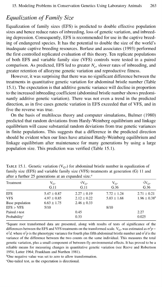
However, it was surprising that there was no significant difference between the
treatments in quantitative genetic variation for abdominal bristle number (Table
15.1). The expectation is that additive genetic variance will decline in proportion
to the increased inbreeding coefficient (abdominal bristle number shows predominantly additive genetic variation). There was not even a trend in the predicted
direction, as in five cases genetic variation in EFS exceeded that of VFS, and in
five the reverse was true.
On the basis of multilocus theory and computer simulations, Bulmer (1980)
predicted that random deviations from Hardy-Weinberg equilibrium and linkage
equilibrium will cause substantial random deviations from true genetic variances
in finite populations. This suggests that a difference in the predicted direction
should be evident when our lines have attained Hardy-Weinberg equilibrium and
linkage equilibrium after maintenance for many generations by using a large
population size. This prediction was verified (Table 15.1).
Table 15.1. Genetic variation (V G* ) for abdominal bristle number in equalization of
family size (EFS) and variable family size (VFS) treatments at generation (G) 11 and
after a further 25 generations at an expanded size.
a
Treatment
V G*
√V G*
V G*
√V G*
G.11
G.11
G.36
G.36
EFS
5.47 ± 0.87
2.27 ± 0.19
7.72 ± 1.24
2.71 ± 0.21
VFS
4.97 ± 0.85
2.12 ± 0.22
5.03 ± 1.68
1.96 ± 0.38
b
Base population
6.63 ± 1.75
2.46 ± 0.33
EFS > VFS
5/10
8/10
Paired t-test
0.45
2.27
Probability
c
0.33
0.025
a Square root transformed data are presented, along with results of tests of significance of the
differences between the EFS and VFS treatments on the transformed scale. V G* was estimated as σ
2
p −
σ
2 d, where σ
2 p is the phenotypic variance for fourth plus fifth abdominal bristle number and σ
2
d is the
variance of the difference between the two counts on the same individual. This measures the total
genetic variation, plus a small component of between-fly environmental effects. It has proved to be a
reliable means for measuring changes in quantitative genetic variation (see Reeve and Robertson
1954; Latter 1964; Frankham and Nurthen 1981).
b One negative value was set to zero to allow transformation.
c One-tailed test, as the expectation is directional.
263
Equalization of Family Size
Equalization of family sizes (EFS) is predicted to double effective population
sizes and hence reduce rates of inbreeding, loss of genetic variation, and inbreeding depression. Consequently, EFS is recommended for use in the captive breeding of endangered species. It has the potential to double the size of the world’s
inadequate captive breeding resources. Borlase and associates (1993) performed
the first controlled replicated evaluation of this theory. Ten replicate populations
of both EFS and variable family size (VFS) controls were tested in a paired
comparison. As predicted, EFS led to greater N e , slower rates of inbreeding, and
greater retention of allozyme genetic variation and reproductive fitness.
However, it was surprising that there was no significant difference between the
treatments in quantitative genetic variation for abdominal bristle number (Table
15.1). The expectation is that additive genetic variance will decline in proportion
to the increased inbreeding coefficient (abdominal bristle number shows predominantly additive genetic variation). There was not even a trend in the predicted
direction, as in five cases genetic variation in EFS exceeded that of VFS, and in
five the reverse was true.
On the basis of multilocus theory and computer simulations, Bulmer (1980)
predicted that random deviations from Hardy-Weinberg equilibrium and linkage
equilibrium will cause substantial random deviations from true genetic variances
in finite populations. This suggests that a difference in the predicted direction
should be evident when our lines have attained Hardy-Weinberg equilibrium and
linkage equilibrium after maintenance for many generations by using a large
population size. This prediction was verified (Table 15.1).
Table 15.1. Genetic variation (V G* ) for abdominal bristle number in equalization of
family size (EFS) and variable family size (VFS) treatments at generation (G) 11 and
after a further 25 generations at an expanded size.
a
Treatment
V G*
√V G*
V G*
√V G*
G.11
G.11
G.36
G.36
EFS
5.47 ± 0.87
2.27 ± 0.19
7.72 ± 1.24
2.71 ± 0.21
VFS
4.97 ± 0.85
2.12 ± 0.22
5.03 ± 1.68
1.96 ± 0.38
b
Base population
6.63 ± 1.75
2.46 ± 0.33
EFS > VFS
5/10
8/10
Paired t-test
0.45
2.27
Probability
c
0.33
0.025
a Square root transformed data are presented, along with results of tests of significance of the
differences between the EFS and VFS treatments on the transformed scale. V G* was estimated as σ
2
p −
σ
2 d, where σ
2 p is the phenotypic variance for fourth plus fifth abdominal bristle number and σ
2
d is the
variance of the difference between the two counts on the same individual. This measures the total
genetic variation, plus a small component of between-fly environmental effects. It has proved to be a
reliable means for measuring changes in quantitative genetic variation (see Reeve and Robertson
1954; Latter 1964; Frankham and Nurthen 1981).
b One negative value was set to zero to allow transformation.
c One-tailed test, as the expectation is directional.