

13. Potential of Branching Processes as a Modeling Tool
205
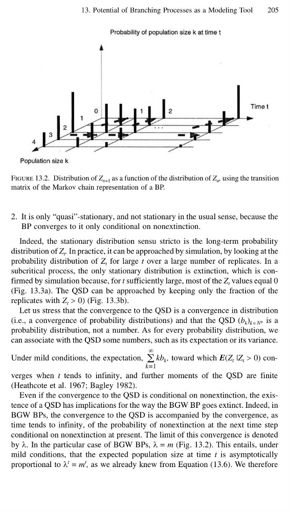
Figure 13.2. Distribution of Z n+1 as a function of the distribution of Z n , using the transition
matrix of the Markov chain representation of a BP.
2. It is only “quasi”-stationary, and not stationary in the usual sense, because the
BP converges to it only conditional on nonextinction.
Indeed, the stationary distribution sensu stricto is the long-term probability
distribution of Z t . In practice, it can be approached by simulation, by looking at the
probability distribution of Z t for large t over a large number of replicates. In a
subcritical process, the only stationary distribution is extinction, which is confirmed by simulation because, for t sufficiently large, most of the Z t values equal 0
(Fig. 13.3a). The QSD can be approached by keeping only the fraction of the
replicates with Z t > 0) (Fig. 13.3b).
Let us stress that the convergence to the QSD is a convergence in distribution
(i.e., a convergence of probability distributions) and that the QSD (b k ) k∈N* is a
probability distribution, not a number. As for every probability distribution, we
can associate with the QSD some numbers, such as its expectation or its variance.
Under mild conditions, the expectation,
∞
͚
k=1
kb k , toward which E(Z t |Z t > 0) converges when t tends to infinity, and further moments of the QSD are finite
(Heathcote et al. 1967; Bagley 1982).
Even if the convergence to the QSD is conditional on nonextinction, the existence of a QSD has implications for the way the BGW BP goes extinct. Indeed, in
BGW BPs, the convergence to the QSD is accompanied by the convergence, as
time tends to infinity, of the probability of nonextinction at the next time step
conditional on nonextinction at present. The limit of this convergence is denoted
by λ. In the particular case of BGW BPs, λ = m (Fig. 13.2). This entails, under
mild conditions, that the expected population size at time t is asymptotically
proportional to λ
t = m
t , as we already knew from Equation (13.6). We therefore
205
Figure 13.2. Distribution of Z n+1 as a function of the distribution of Z n , using the transition
matrix of the Markov chain representation of a BP.
2. It is only “quasi”-stationary, and not stationary in the usual sense, because the
BP converges to it only conditional on nonextinction.
Indeed, the stationary distribution sensu stricto is the long-term probability
distribution of Z t . In practice, it can be approached by simulation, by looking at the
probability distribution of Z t for large t over a large number of replicates. In a
subcritical process, the only stationary distribution is extinction, which is confirmed by simulation because, for t sufficiently large, most of the Z t values equal 0
(Fig. 13.3a). The QSD can be approached by keeping only the fraction of the
replicates with Z t > 0) (Fig. 13.3b).
Let us stress that the convergence to the QSD is a convergence in distribution
(i.e., a convergence of probability distributions) and that the QSD (b k ) k∈N* is a
probability distribution, not a number. As for every probability distribution, we
can associate with the QSD some numbers, such as its expectation or its variance.
Under mild conditions, the expectation,
∞
͚
k=1
kb k , toward which E(Z t |Z t > 0) converges when t tends to infinity, and further moments of the QSD are finite
(Heathcote et al. 1967; Bagley 1982).
Even if the convergence to the QSD is conditional on nonextinction, the existence of a QSD has implications for the way the BGW BP goes extinct. Indeed, in
BGW BPs, the convergence to the QSD is accompanied by the convergence, as
time tends to infinity, of the probability of nonextinction at the next time step
conditional on nonextinction at present. The limit of this convergence is denoted
by λ. In the particular case of BGW BPs, λ = m (Fig. 13.2). This entails, under
mild conditions, that the expected population size at time t is asymptotically
proportional to λ
t = m
t , as we already knew from Equation (13.6). We therefore