

9. Assessing Land-Use Impacts on Bull Trout Using Bayesian Belief Networks
135
where N i = the redd count in year i, ˜
N= the equilibrium attraction point (i.e., the
count at which the expectation of N t+1 = N t ), g = density-dependent scaling
parameter, and ε = normally distributed error term with zero mean and standard
deviation, s(N t ). For simulation purposes, s(N t ) is defined as
σ
s(N t ) =
(9.5)
1 +
N t − ˜
N
γ ˜
N
if N t > ˜
N, and s(N t ) = σ otherwise. This adjustment in the error term imposes
higher fidelity to the density-dependent control at high population levels and tends
to suppress large unreasonable values from occurring during simulation.
Parameter estimates were obtained by using linear regression and Dennis and
Taper’s (1994) version of the model:
ln
N t+1
N t = a + bN t + ε
(9.6)
where a = 1/ γ, and b = −1/ γ ˜
N, and ε is a normally distributed error term with zero
mean and standard deviation, s(N). As Dennis and Taper (1994) note, point
estimates obtained in this manner are appropriate, although hypothesis testing
based on linear regression estimates of the error terms would be invalid due to the
autoregressive structure of the model.
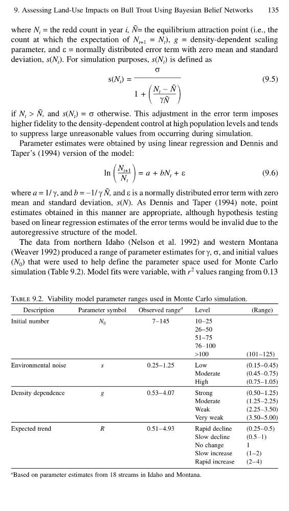
The data from northern Idaho (Nelson et al. 1992) and western Montana
(Weaver 1992) produced a range of parameter estimates for γ, σ, and initial values
(N 0 ) that were used to help define the parameter space used for Monte Carlo
simulation (Table 9.2). Model fits were variable, with r
2 values ranging from 0.13
Table 9.2. Viability model parameter ranges used in Monte Carlo simulation.
Description
Parameter symbol
Observed range
a
Level
(Range)
Initial number
N 0
7–145
10–25
26–50
51–75
76–100
>100
(101–125)
Environmental noise
s
0.25–1.25
Low
(0.15–0.45)
Moderate
(0.45–0.75)
High
(0.75–1.05)
Density dependence
g
0.53– 4.07
Strong
(0.50–1.25)
Moderate
(1.25–2.25)
Weak
(2.25–3.50)
Very weak
(3.50–5.00)
Expected trend
R
0.51– 4.93
Rapid decline
(0.25–0.5)
Slow decline
(0.5–1)
No change
1
Slow increase
(1–2)
Rapid increase
(2– 4)
a Based on parameter estimates from 18 streams in Idaho and Montana.
135
where N i = the redd count in year i, ˜
N= the equilibrium attraction point (i.e., the
count at which the expectation of N t+1 = N t ), g = density-dependent scaling
parameter, and ε = normally distributed error term with zero mean and standard
deviation, s(N t ). For simulation purposes, s(N t ) is defined as
σ
s(N t ) =
(9.5)
1 +
N t − ˜
N
γ ˜
N
if N t > ˜
N, and s(N t ) = σ otherwise. This adjustment in the error term imposes
higher fidelity to the density-dependent control at high population levels and tends
to suppress large unreasonable values from occurring during simulation.
Parameter estimates were obtained by using linear regression and Dennis and
Taper’s (1994) version of the model:
ln
N t+1
N t = a + bN t + ε
(9.6)
where a = 1/ γ, and b = −1/ γ ˜
N, and ε is a normally distributed error term with zero
mean and standard deviation, s(N). As Dennis and Taper (1994) note, point
estimates obtained in this manner are appropriate, although hypothesis testing
based on linear regression estimates of the error terms would be invalid due to the
autoregressive structure of the model.
The data from northern Idaho (Nelson et al. 1992) and western Montana
(Weaver 1992) produced a range of parameter estimates for γ, σ, and initial values
(N 0 ) that were used to help define the parameter space used for Monte Carlo
simulation (Table 9.2). Model fits were variable, with r
2 values ranging from 0.13
Table 9.2. Viability model parameter ranges used in Monte Carlo simulation.
Description
Parameter symbol
Observed range
a
Level
(Range)
Initial number
N 0
7–145
10–25
26–50
51–75
76–100
>100
(101–125)
Environmental noise
s
0.25–1.25
Low
(0.15–0.45)
Moderate
(0.45–0.75)
High
(0.75–1.05)
Density dependence
g
0.53– 4.07
Strong
(0.50–1.25)
Moderate
(1.25–2.25)
Weak
(2.25–3.50)
Very weak
(3.50–5.00)
Expected trend
R
0.51– 4.93
Rapid decline
(0.25–0.5)
Slow decline
(0.5–1)
No change
1
Slow increase
(1–2)
Rapid increase
(2– 4)
a Based on parameter estimates from 18 streams in Idaho and Montana.