

26
J. Lou· T. Wolf· W. Rosenthal
c = {allW + a23W~ (OU + °oV)}e + a21W~ °oe + a22W uh ooe
Ws ox 9'
Ws t
Ws x
+ ad~)-- - a2IW-- ex- - a2IW-- e - ,
vh oe
h 0 ( oe)
h 0 ( oe)
Ws oy
Ws ox ox
Ws oy Y oy
(9)
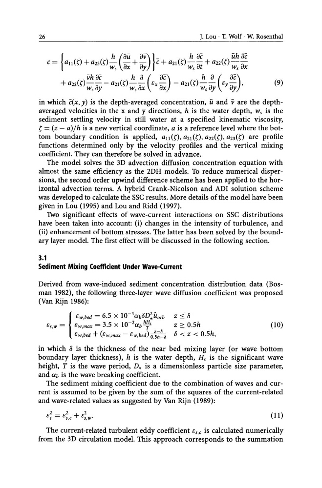
in which e(x,y) is the depth-averaged concentration, u and v are the depthaveraged velocities in the x and y directions, h is the water depth, Ws is the
sediment settling velocity in still water at a specified kinematic viscosity,
~ = (z - a)jh is a new vertical coordinate, a is a reference level where the bottom boundary condition is applied, all W, a2l W, a22W, a23W are profile
functions determined only by the velocity profiles and the vertical mixing
coefficient. They can therefore be solved in advance.
The model solves the 3D advection diffusion concentration equation with
almost the same efficiency as the 2DH models. To reduce numerical dispersions, the second order upwind difference scheme has been applied to the horizontal advection terms. A hybrid Crank-Nicolson and ADI solution scheme
was developed to calculate the SSC results. More details of the model have been
given in Lou (1995) and Lou and Ridd (1997).
Two significant effects of wave-current interactions on SSC distributions
have been taken into account: (i) changes in the intensity of turbulence, and
(ii) enhancement of bottom stresses. The latter has been solved by the boundary layer model. The first effect will be discussed in the following section.
3.1
Sediment Mixing Coefficient Under Wave-Current
Derived from wave-induced sediment concentration distribution data (Bosman 1982), the following three-layer wave diffusion coefficient was proposed
(Van Rijn 1986):
z~/)
z:::: O.sh
/) < z < O.Sh,
(10)
in which /) is the thickness of the near bed mixing layer (or wave bottom
boundary layer thickness), h is the water depth, Hs is the significant wave
height, T is the wave period, D* is a dimensionless particle size parameter,
and CXb is the wave breaking coefficient.
The sediment mixing coefficient due to the combination of waves and current is assumed to be given by the sum of the squares of the current-related
and wave-related values as suggested by Van Rijn (1989):
(11)
The current-related turbulent eddy coefficient es,c is calculated numerically
from the 3D circulation model. This approach corresponds to the summation
J. Lou· T. Wolf· W. Rosenthal
c = {allW + a23W~ (OU + °oV)}e + a21W~ °oe + a22W uh ooe
Ws ox 9'
Ws t
Ws x
+ ad~)-- - a2IW-- ex- - a2IW-- e - ,
vh oe
h 0 ( oe)
h 0 ( oe)
Ws oy
Ws ox ox
Ws oy Y oy
(9)
in which e(x,y) is the depth-averaged concentration, u and v are the depthaveraged velocities in the x and y directions, h is the water depth, Ws is the
sediment settling velocity in still water at a specified kinematic viscosity,
~ = (z - a)jh is a new vertical coordinate, a is a reference level where the bottom boundary condition is applied, all W, a2l W, a22W, a23W are profile
functions determined only by the velocity profiles and the vertical mixing
coefficient. They can therefore be solved in advance.
The model solves the 3D advection diffusion concentration equation with
almost the same efficiency as the 2DH models. To reduce numerical dispersions, the second order upwind difference scheme has been applied to the horizontal advection terms. A hybrid Crank-Nicolson and ADI solution scheme
was developed to calculate the SSC results. More details of the model have been
given in Lou (1995) and Lou and Ridd (1997).
Two significant effects of wave-current interactions on SSC distributions
have been taken into account: (i) changes in the intensity of turbulence, and
(ii) enhancement of bottom stresses. The latter has been solved by the boundary layer model. The first effect will be discussed in the following section.
3.1
Sediment Mixing Coefficient Under Wave-Current
Derived from wave-induced sediment concentration distribution data (Bosman 1982), the following three-layer wave diffusion coefficient was proposed
(Van Rijn 1986):
z~/)
z:::: O.sh
/) < z < O.Sh,
(10)
in which /) is the thickness of the near bed mixing layer (or wave bottom
boundary layer thickness), h is the water depth, Hs is the significant wave
height, T is the wave period, D* is a dimensionless particle size parameter,
and CXb is the wave breaking coefficient.
The sediment mixing coefficient due to the combination of waves and current is assumed to be given by the sum of the squares of the current-related
and wave-related values as suggested by Van Rijn (1989):
(11)
The current-related turbulent eddy coefficient es,c is calculated numerically
from the 3D circulation model. This approach corresponds to the summation