

Lagrangian Modelling Techniques Simulating Wave and Sediment Dynamics ...
9
I
J 0 r i I
r- - '~
0""""
'"
2
~
. .
w
;
C6
.,
;
o l:r..lt SINse.
1
1
0<
~
(el
§
•
~
02
c..
~
'"
00
0
~
Ot,DWt"'5(H~
Z
<>
0
0
"
5
0
~
0.
0
I (01
o
0
15
~
0.0
o.
I
1000,0
0'
1
~
BOO 0
o C:. J ( II,.!II"
"
0<
b C: . U '114.9~)
<>
OJ
GOO 0
• C.J 'll!U~}
W
!
:r
02
'00 0
'"
,.
o i
200,0
;
8
00
0.0
2'~2
2160
" . .
211S
2184
2152
o
IWil:sr I'fuwS[IIt
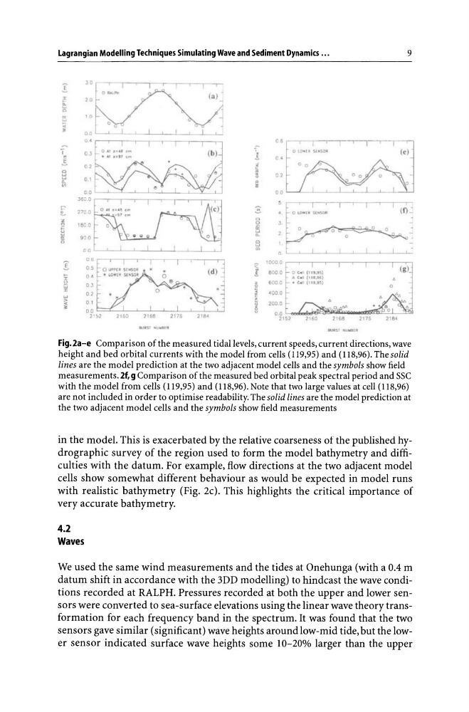
Fig.2a-e Comparison of the measured tidal levels, current speeds, current directions, wave
height and bed orbital currents with the model from cells (119,95) and (I 18,96). The solid
lines are the model prediction at the two adjacent model cells and the symbols show field
measurements. 2f, g Comparison of the measured bed orbital peak spectral period and SSC
with the model from cells (I 19,95) and (I 18,96). Note that two large values at cell (118,96)
are not included in order to optimise readability. The solid lines are the model prediction at
the two adjacent model cells and the symbols show field measurements
in the model. This is exacerbated by the relative coarseness of the published hydrographic survey of the region used to form the model bathymetry and difficulties with the datum. For example, flow directions at the two adjacent model
cells show somewhat different behaviour as would be expected in model runs
with realistic bathymetry (Fig. 2c). This highlights the critical importance of
very accurate bathymetry.
4.2
Waves
We used the same wind measurements and the tides at Onehunga (with a 0.4 m
datum shift in accordance with the 3DD modelling) to hindcast the wave conditions recorded at RALPH. Pressures recorded at both the upper and lower sensors were converted to sea -surface elevations using the linear wave theory transformation for each frequency band in the spectrum. It was found that the two
sensors gave similar (significant) wave heights around low-mid tide, but the lower sensor indicated surface wave heights some 10-20% larger than the upper
9
I
J 0 r i I
r- - '~
0""""
'"
2
~
. .
w
;
C6
.,
;
o l:r..lt SINse.
1
1
0<
~
(el
§
•
~
02
c..
~
'"
00
0
~
Ot,DWt"'5(H~
Z
<>
0
0
"
5
0
~
0.
0
I (01
o
0
15
~
0.0
o.
I
1000,0
0'
1
~
BOO 0
o C:. J ( II,.!II"
"
0<
b C: . U '114.9~)
<>
OJ
GOO 0
• C.J 'll!U~}
W
!
:r
02
'00 0
'"
,.
o i
200,0
;
8
00
0.0
2'~2
2160
" . .
211S
2184
2152
o
IWil:sr I'fuwS[IIt
Fig.2a-e Comparison of the measured tidal levels, current speeds, current directions, wave
height and bed orbital currents with the model from cells (119,95) and (I 18,96). The solid
lines are the model prediction at the two adjacent model cells and the symbols show field
measurements. 2f, g Comparison of the measured bed orbital peak spectral period and SSC
with the model from cells (I 19,95) and (I 18,96). Note that two large values at cell (118,96)
are not included in order to optimise readability. The solid lines are the model prediction at
the two adjacent model cells and the symbols show field measurements
in the model. This is exacerbated by the relative coarseness of the published hydrographic survey of the region used to form the model bathymetry and difficulties with the datum. For example, flow directions at the two adjacent model
cells show somewhat different behaviour as would be expected in model runs
with realistic bathymetry (Fig. 2c). This highlights the critical importance of
very accurate bathymetry.
4.2
Waves
We used the same wind measurements and the tides at Onehunga (with a 0.4 m
datum shift in accordance with the 3DD modelling) to hindcast the wave conditions recorded at RALPH. Pressures recorded at both the upper and lower sensors were converted to sea -surface elevations using the linear wave theory transformation for each frequency band in the spectrum. It was found that the two
sensors gave similar (significant) wave heights around low-mid tide, but the lower sensor indicated surface wave heights some 10-20% larger than the upper