

72
S. LI, Z. CHENG, AND W.P. WEEKS
4.2.1
Ice Motion Products
The overall operating system at the Alaska SAR Facility (ASF) includes a Geophysical
Processor System (GPS) designed by the Jet Propulsion Laboratory (JPL) of the California Institute of Technology (Kwok et al. 1990; McConnell et al. 1991; Kwok and Pang
1992). This system produces a description of the movement field as specified by the
motions of identifiable ice features in terms of their initial and final geographical positions and the displacements of individual ice motion vectors between two sequential
SAR images. The system is able to derive correct ice motion vectors even if ice floes
experience both translation and rotation.
By convention, the initial image is referred to as the "source image" and the final image
as the "target image:' In order to carry out this procedure, a special polar stereo graphic
map projection (SSM/I) is used to generate a unique 2-D Cartesian system onto which all
the ice motion vectors are mapped. The basic units of 5X5 km square grid cells are obtained
from a uniformly spaced grid on the source image. Ice motion is then tracked by a bestmatch of the ice features in each initial source grid cell with the positions of the same features in the target image. The initial and final positions of the center of each grid cell provide a pair of tie points that define a specific ice motion vector. The ice motion vector can
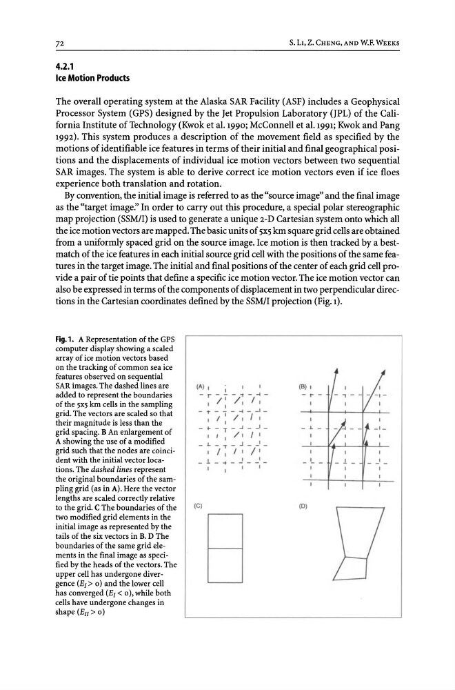
also be expressed in terms of the components of displacement in two perpendicular directions in the Cartesian coordinates defined by the SSM/I projection (Fig. 1).
Fig.1. A Representation of the GPS
computer display showing a scaled
array of ice motion vectors based
on the tracking of common sea ice
features observed on sequential
SAR images. The dashed lines are
added to represent the boundaries
of the 5X5 km cells in the sampling
grid. The vectors are scaled so that
their magnitude is less than the
grid spacing. B An enlargement of
A showing the use of a modified
grid such that the nodes are coincident with the initial vector locations. The dashed lines represent
the original boundaries of the sampling grid (as in A). Here the vector
lengths are scaled correctly relative
to the grid. C The boundaries of the
two modified grid elements in the
initial image as represented by the
tails of the six vectors in B. D The
boundaries of the same grid elements in the final image as specified by the heads of the vectors. The
upper cell has undergone divergence (EI> 0) and the lower cell
has converged (E1 < 0), while both
cells have undergone changes in
shape (Ell> 0)
(A) ,
,
I
- r - - - ~ - ~ -
I
/
'
/ ,
I ,
,
- ~ - - - ~ - _II
I ' / I I ,
,
- ~ - T - ~ - J -
,
I
,
/ , I I
- ~ - T - J - ~ -
, I I I , / I
,
,
I
- - - ~ - - - - -
,
,
I
(C)
(8) ,
- ,.. -
- ~ -
,
_ ':.. _
_ 1 _
_ _I _
(0)
S. LI, Z. CHENG, AND W.P. WEEKS
4.2.1
Ice Motion Products
The overall operating system at the Alaska SAR Facility (ASF) includes a Geophysical
Processor System (GPS) designed by the Jet Propulsion Laboratory (JPL) of the California Institute of Technology (Kwok et al. 1990; McConnell et al. 1991; Kwok and Pang
1992). This system produces a description of the movement field as specified by the
motions of identifiable ice features in terms of their initial and final geographical positions and the displacements of individual ice motion vectors between two sequential
SAR images. The system is able to derive correct ice motion vectors even if ice floes
experience both translation and rotation.
By convention, the initial image is referred to as the "source image" and the final image
as the "target image:' In order to carry out this procedure, a special polar stereo graphic
map projection (SSM/I) is used to generate a unique 2-D Cartesian system onto which all
the ice motion vectors are mapped. The basic units of 5X5 km square grid cells are obtained
from a uniformly spaced grid on the source image. Ice motion is then tracked by a bestmatch of the ice features in each initial source grid cell with the positions of the same features in the target image. The initial and final positions of the center of each grid cell provide a pair of tie points that define a specific ice motion vector. The ice motion vector can
also be expressed in terms of the components of displacement in two perpendicular directions in the Cartesian coordinates defined by the SSM/I projection (Fig. 1).
Fig.1. A Representation of the GPS
computer display showing a scaled
array of ice motion vectors based
on the tracking of common sea ice
features observed on sequential
SAR images. The dashed lines are
added to represent the boundaries
of the 5X5 km cells in the sampling
grid. The vectors are scaled so that
their magnitude is less than the
grid spacing. B An enlargement of
A showing the use of a modified
grid such that the nodes are coincident with the initial vector locations. The dashed lines represent
the original boundaries of the sampling grid (as in A). Here the vector
lengths are scaled correctly relative
to the grid. C The boundaries of the
two modified grid elements in the
initial image as represented by the
tails of the six vectors in B. D The
boundaries of the same grid elements in the final image as specified by the heads of the vectors. The
upper cell has undergone divergence (EI> 0) and the lower cell
has converged (E1 < 0), while both
cells have undergone changes in
shape (Ell> 0)
(A) ,
,
I
- r - - - ~ - ~ -
I
/
'
/ ,
I ,
,
- ~ - - - ~ - _II
I ' / I I ,
,
- ~ - T - ~ - J -
,
I
,
/ , I I
- ~ - T - J - ~ -
, I I I , / I
,
,
I
- - - ~ - - - - -
,
,
I
(C)
(8) ,
- ,.. -
- ~ -
,
_ ':.. _
_ 1 _
_ _I _
(0)