

62
STEPHEN GRIFFIES
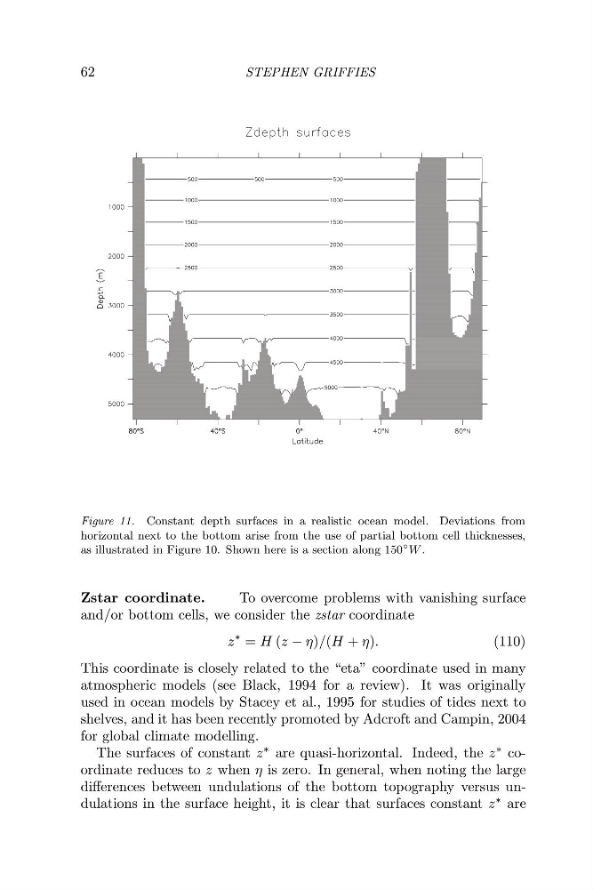
Figure 11. Constant depth surfaces in a realistic ocean model. Deviations from
horizontal next to the bottom arise from the use of partial bottom cell thicknesses,
as illustrated in Figure 10. Shown here is a section along 150
◦ W .
Zstar coordinate.
To overcome problems with vanishing surface
and/or bottom cells, we consider the zstar coordinate
z
∗ = H (z − η)/(H + η).
(110)
This coordinate is closely related to the “eta” coordinate used in many
atmospheric models (see Black, 1994 for a review). It was originally
used in ocean models by Stacey et al., 1995 for studies of tides next to
shelves, and it has been recently promoted by Adcroft and Campin, 2004
for global climate modelling.
The surfaces of constant z ∗ are quasi-horizontal. Indeed, the z ∗ coordinate reduces to z when η is zero. In general, when noting the large
differences between undulations of the bottom topography versus undulations in the surface height, it is clear that surfaces constant z ∗ are
STEPHEN GRIFFIES
Figure 11. Constant depth surfaces in a realistic ocean model. Deviations from
horizontal next to the bottom arise from the use of partial bottom cell thicknesses,
as illustrated in Figure 10. Shown here is a section along 150
◦ W .
Zstar coordinate.
To overcome problems with vanishing surface
and/or bottom cells, we consider the zstar coordinate
z
∗ = H (z − η)/(H + η).
(110)
This coordinate is closely related to the “eta” coordinate used in many
atmospheric models (see Black, 1994 for a review). It was originally
used in ocean models by Stacey et al., 1995 for studies of tides next to
shelves, and it has been recently promoted by Adcroft and Campin, 2004
for global climate modelling.
The surfaces of constant z ∗ are quasi-horizontal. Indeed, the z ∗ coordinate reduces to z when η is zero. In general, when noting the large
differences between undulations of the bottom topography versus undulations in the surface height, it is clear that surfaces constant z ∗ are