

56
STEPHEN GRIFFIES
5.
The pressure force
A hydrostatic fluid maintains the balance p,, = -pg. This balance
means that the pressure at a point in a hydrostatic fluid is determined
by the weight of fluid above this point. This relation is maintained quite
well in the ocean on spatial scales larger than roughly lkm. Precisely,
when the squared ratio of the vertical to horizontal scales of motion is
small, then the hydrostatic approximation is well maintained. In this
case, the vertical momentum budget reduces to the hydrostatic balance,
in which case vertical acceleration and friction are neglected. If we are
interested in explicitly representing such motions as Kelvin-Helmholtz
billows and flow within a convective chimney, vertical accelerations are
nontrivial and so the non-hydrostatic momentum budget must be used.
The hydrostatic balance greatly affects the algorithms used to numerically solve the equations of motion. The paper by Marshall et al., 1997
highlights these points in the context of developing an algorithm suited
for both hydrostatic and non-hydrostatic simulations. However, so far in
ocean modelling, no global simulations have been run at resolutions sufficiently refined to require the non-hydrostatic equations. Additionally,
many regional and coastal models, even some with resolutions refined
smaller than lkm, still maintain the hydrostatic approximation, and thus
they must parameterize the unrepresented non-hydrostatic motions.
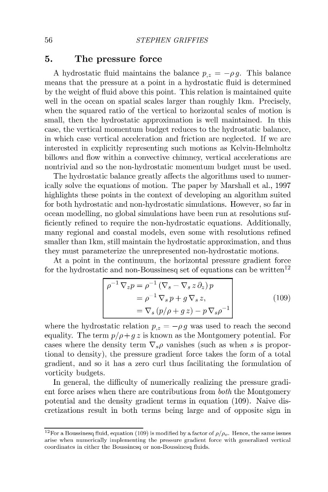
At a point in the continuum, the horizontal pressure gradient force
for the hydrostatic and non-Boussinesq set of equations can be written12
p-l V,p = p-I (V, - V, z 8,) p
= P - l v , p + g V , z ,
= Vs(PlP+gz) -PV,P
- 1
where the hydrostatic relation p,, = -pg was used to reach the second
equality. The term plp + g z is known as the Montgomery potential. For
cases where the density term V,p vanishes (such as when s is proportional to density), the pressure gradient force takes the form of a total
gradient, and so it has a zero curl thus facilitating the formulation of
vorticity budgets.
In general, the difficulty of numerically realizing the pressure gradient force arises when there are contributions from both the Montgomery
potential and the density gradient terms in equation (109). Naive discretization~ result in both terms being large and of opposite sign in
1 2 ~ o r
a Boussinesq fluid, equation (109) is modified by a factor of pip,. Hence, the same issues
arise when numerically implementing the pressure gradient force with generalized vertical
coordinates in either the Boussinesq or non-Boussinesq fluids.
STEPHEN GRIFFIES
5.
The pressure force
A hydrostatic fluid maintains the balance p,, = -pg. This balance
means that the pressure at a point in a hydrostatic fluid is determined
by the weight of fluid above this point. This relation is maintained quite
well in the ocean on spatial scales larger than roughly lkm. Precisely,
when the squared ratio of the vertical to horizontal scales of motion is
small, then the hydrostatic approximation is well maintained. In this
case, the vertical momentum budget reduces to the hydrostatic balance,
in which case vertical acceleration and friction are neglected. If we are
interested in explicitly representing such motions as Kelvin-Helmholtz
billows and flow within a convective chimney, vertical accelerations are
nontrivial and so the non-hydrostatic momentum budget must be used.
The hydrostatic balance greatly affects the algorithms used to numerically solve the equations of motion. The paper by Marshall et al., 1997
highlights these points in the context of developing an algorithm suited
for both hydrostatic and non-hydrostatic simulations. However, so far in
ocean modelling, no global simulations have been run at resolutions sufficiently refined to require the non-hydrostatic equations. Additionally,
many regional and coastal models, even some with resolutions refined
smaller than lkm, still maintain the hydrostatic approximation, and thus
they must parameterize the unrepresented non-hydrostatic motions.
At a point in the continuum, the horizontal pressure gradient force
for the hydrostatic and non-Boussinesq set of equations can be written12
p-l V,p = p-I (V, - V, z 8,) p
= P - l v , p + g V , z ,
= Vs(PlP+gz) -PV,P
- 1
where the hydrostatic relation p,, = -pg was used to reach the second
equality. The term plp + g z is known as the Montgomery potential. For
cases where the density term V,p vanishes (such as when s is proportional to density), the pressure gradient force takes the form of a total
gradient, and so it has a zero curl thus facilitating the formulation of
vorticity budgets.
In general, the difficulty of numerically realizing the pressure gradient force arises when there are contributions from both the Montgomery
potential and the density gradient terms in equation (109). Naive discretization~ result in both terms being large and of opposite sign in
1 2 ~ o r
a Boussinesq fluid, equation (109) is modified by a factor of pip,. Hence, the same issues
arise when numerically implementing the pressure gradient force with generalized vertical
coordinates in either the Boussinesq or non-Boussinesq fluids.