

538
ANDREAS OSCHLIES
the often expensive computation of the gradient. In the following, a
brief overview will be given of methods that have so far been applied to
marine ecosystem models.
Gradient descent methods.
A standard conjugate gradient
method, that alters search directions in consecutive iterations, has been
applied by Fasham and Evans [1995] to optimise a model at the site
of the North Atlantic Bloom Experiment (47 ◦ N, 20 ◦ W). The cost function’s gradient was approximated by varying the individual parameters
by a finite amount and computing the corresponding difference quotient.
A finite-difference approximation of the cost function gradient was also
used by Prunet et al. [1996a,b]. It is generally and without detailed
investigation assumed that the cost function is smooth enough so that
the estimated gradient (times −1) points at least downward in the cost
function topography and that errors in its exact direction and size will
only slow, but not hinder, convergence of the descent algorithm. Prunet
et al. [1996a,b] in addition made the probably more critical assumption
of a locally parabolic shape of the cost function at each iteration of a
gradient descent method. Their sensitivity analysis indicated that this
method did not generally yield robust parameter estimates, and that
posterior error estimates were too small compared to the results of their
sensitivity experiments.
In order to improve the quality of the gradient computation, the adjoint method has received considerable attention. It was first used in
the context of marine ecosystem models by Lawson et al. [1995]. The
adjoint method computes the exact gradient of the cost function J(p)
by resorting to the method of Langrangian multipliers. This method has
been widely used in statistical mechanics to derive the Euler-Lagrange
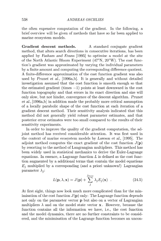
equations. In essence, a Lagrange function L is defined as the cost function augmented by a additional terms that contain the model equations
E j multiplied by a corresponding (and a priori unknown!) Lagrangian
parameter λ j :
L(p, λ, x) = J(p) +
jmax
j
λ j E j (x) .
(24.5)
At first sight, things now look much more complicated than for the minimisation of the cost function J(p) only: The Lagrange function depends
not only on the parameter vector p but also on a vector of Lagrangian
multipliers λ and on the model state vector x . However, because the
function contains all the information we have, i.e., the cost function
and the model dynamics, there are no further constraints to be considered, and the minimisation of the Lagrange function becomes an uncon,
,
,
ANDREAS OSCHLIES
the often expensive computation of the gradient. In the following, a
brief overview will be given of methods that have so far been applied to
marine ecosystem models.
Gradient descent methods.
A standard conjugate gradient
method, that alters search directions in consecutive iterations, has been
applied by Fasham and Evans [1995] to optimise a model at the site
of the North Atlantic Bloom Experiment (47 ◦ N, 20 ◦ W). The cost function’s gradient was approximated by varying the individual parameters
by a finite amount and computing the corresponding difference quotient.
A finite-difference approximation of the cost function gradient was also
used by Prunet et al. [1996a,b]. It is generally and without detailed
investigation assumed that the cost function is smooth enough so that
the estimated gradient (times −1) points at least downward in the cost
function topography and that errors in its exact direction and size will
only slow, but not hinder, convergence of the descent algorithm. Prunet
et al. [1996a,b] in addition made the probably more critical assumption
of a locally parabolic shape of the cost function at each iteration of a
gradient descent method. Their sensitivity analysis indicated that this
method did not generally yield robust parameter estimates, and that
posterior error estimates were too small compared to the results of their
sensitivity experiments.
In order to improve the quality of the gradient computation, the adjoint method has received considerable attention. It was first used in
the context of marine ecosystem models by Lawson et al. [1995]. The
adjoint method computes the exact gradient of the cost function J(p)
by resorting to the method of Langrangian multipliers. This method has
been widely used in statistical mechanics to derive the Euler-Lagrange
equations. In essence, a Lagrange function L is defined as the cost function augmented by a additional terms that contain the model equations
E j multiplied by a corresponding (and a priori unknown!) Lagrangian
parameter λ j :
L(p, λ, x) = J(p) +
jmax
j
λ j E j (x) .
(24.5)
At first sight, things now look much more complicated than for the minimisation of the cost function J(p) only: The Lagrange function depends
not only on the parameter vector p but also on a vector of Lagrangian
multipliers λ and on the model state vector x . However, because the
function contains all the information we have, i.e., the cost function
and the model dynamics, there are no further constraints to be considered, and the minimisation of the Lagrange function becomes an uncon,
,
,