

534
ANDREAS OSCHLIES
5.
Data assimilation methods used in marine
biogeochemical modelling
5.1
Sequential methods
Sequential assimilation methods are constructed to accumulate information gathered from both observations and model predictions in time
with the aim to generate an optimal state estimate. This approach is
widely used in operational systems for which fast and robust delivery
of information is a crucial aspect, ranging from instrument-guided aircraft landing, and related less peaceful applications, to atmospheric and
oceanic weather forecasting. Most methods are approximations to, or
descendants of, the Kalman Filter [Kalman, 1960]. Its basic principle is
that of optimal interpolation between an observation and its simulated
counterpart.
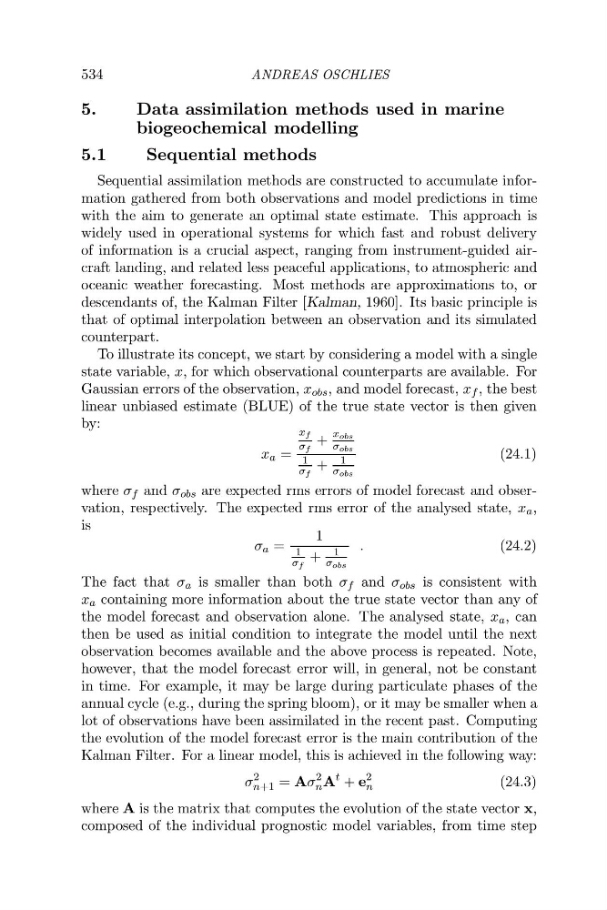
To illustrate its concept, we start by considering a model with a single
state variable, x, for which observational counterparts are available. For
Gaussian errors of the observation, x obs , and model forecast, x f , the best
linear unbiased estimate (BLUE) of the true state vector is then given
by:
x a =
x f
σ f
+
x obs
σ obs
1
σ f
+
1
σ obs
(24.1)
where σ f and σ obs are expected rms errors of model forecast and observation, respectively. The expected rms error of the analysed state, x a ,
is
σ a =
1
1
σ f
+
1
σ obs
.
(24.2)
The fact that σ a is smaller than both σ f and σ obs is consistent with
x a containing more information about the true state vector than any of
the model forecast and observation alone. The analysed state, x a , can
then be used as initial condition to integrate the model until the next
observation becomes available and the above process is repeated. Note,
however, that the model forecast error will, in general, not be constant
in time. For example, it may be large during particulate phases of the
annual cycle (e.g., during the spring bloom), or it may be smaller when a
lot of observations have been assimilated in the recent past. Computing
the evolution of the model forecast error is the main contribution of the
Kalman Filter. For a linear model, this is achieved in the following way:
σ
2
n+1 = Aσ
2
n A
t + e
2
n
(24.3)
where A is the matrix that computes the evolution of the state vector x,
composed of the individual prognostic model variables, from time step
ANDREAS OSCHLIES
5.
Data assimilation methods used in marine
biogeochemical modelling
5.1
Sequential methods
Sequential assimilation methods are constructed to accumulate information gathered from both observations and model predictions in time
with the aim to generate an optimal state estimate. This approach is
widely used in operational systems for which fast and robust delivery
of information is a crucial aspect, ranging from instrument-guided aircraft landing, and related less peaceful applications, to atmospheric and
oceanic weather forecasting. Most methods are approximations to, or
descendants of, the Kalman Filter [Kalman, 1960]. Its basic principle is
that of optimal interpolation between an observation and its simulated
counterpart.
To illustrate its concept, we start by considering a model with a single
state variable, x, for which observational counterparts are available. For
Gaussian errors of the observation, x obs , and model forecast, x f , the best
linear unbiased estimate (BLUE) of the true state vector is then given
by:
x a =
x f
σ f
+
x obs
σ obs
1
σ f
+
1
σ obs
(24.1)
where σ f and σ obs are expected rms errors of model forecast and observation, respectively. The expected rms error of the analysed state, x a ,
is
σ a =
1
1
σ f
+
1
σ obs
.
(24.2)
The fact that σ a is smaller than both σ f and σ obs is consistent with
x a containing more information about the true state vector than any of
the model forecast and observation alone. The analysed state, x a , can
then be used as initial condition to integrate the model until the next
observation becomes available and the above process is repeated. Note,
however, that the model forecast error will, in general, not be constant
in time. For example, it may be large during particulate phases of the
annual cycle (e.g., during the spring bloom), or it may be smaller when a
lot of observations have been assimilated in the recent past. Computing
the evolution of the model forecast error is the main contribution of the
Kalman Filter. For a linear model, this is achieved in the following way:
σ
2
n+1 = Aσ
2
n A
t + e
2
n
(24.3)
where A is the matrix that computes the evolution of the state vector x,
composed of the individual prognostic model variables, from time step