

SOME OCEAN MODEL FUNDAMENTALS
27
ments commonly used for regional and global models. Such could
represent a major advance in ocean modelling.
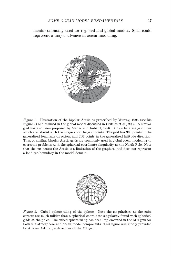
Figure 1. Illustration of the bipolar Arctic as prescribed by Murray, 1996 (see his
Figure 7) and realized in the global model discussed in Griffies et al., 2005. A similar
grid has also been proposed by Madec and Imbard, 1996. Shown here are grid lines
which are labeled with the integers for the grid points. The grid has 360 points in the
generalized longitude direction, and 200 points in the generalized latitude direction.
This, or similar, bipolar Arctic grids are commonly used in global ocean modelling to
overcome problems with the spherical coordinate singularity at the North Pole. Note
that the cut across the Arctic is a limitation of the graphics, and does not represent
a land-sea boundary in the model domain.
Figure 2. Cubed sphere tiling of the sphere. Note the singularities at the cube
corners are much milder than a spherical coordinate singularity found with spherical
grids at the poles. The cubed sphere tiling has been implemented in the MITgcm for
both the atmosphere and ocean model components. This figure was kindly provided
by Alistair Adcroft, a developer of the MITgcm.
27
ments commonly used for regional and global models. Such could
represent a major advance in ocean modelling.
Figure 1. Illustration of the bipolar Arctic as prescribed by Murray, 1996 (see his
Figure 7) and realized in the global model discussed in Griffies et al., 2005. A similar
grid has also been proposed by Madec and Imbard, 1996. Shown here are grid lines
which are labeled with the integers for the grid points. The grid has 360 points in the
generalized longitude direction, and 200 points in the generalized latitude direction.
This, or similar, bipolar Arctic grids are commonly used in global ocean modelling to
overcome problems with the spherical coordinate singularity at the North Pole. Note
that the cut across the Arctic is a limitation of the graphics, and does not represent
a land-sea boundary in the model domain.
Figure 2. Cubed sphere tiling of the sphere. Note the singularities at the cube
corners are much milder than a spherical coordinate singularity found with spherical
grids at the poles. The cubed sphere tiling has been implemented in the MITgcm for
both the atmosphere and ocean model components. This figure was kindly provided
by Alistair Adcroft, a developer of the MITgcm.