

350
FLORENCE RABIER
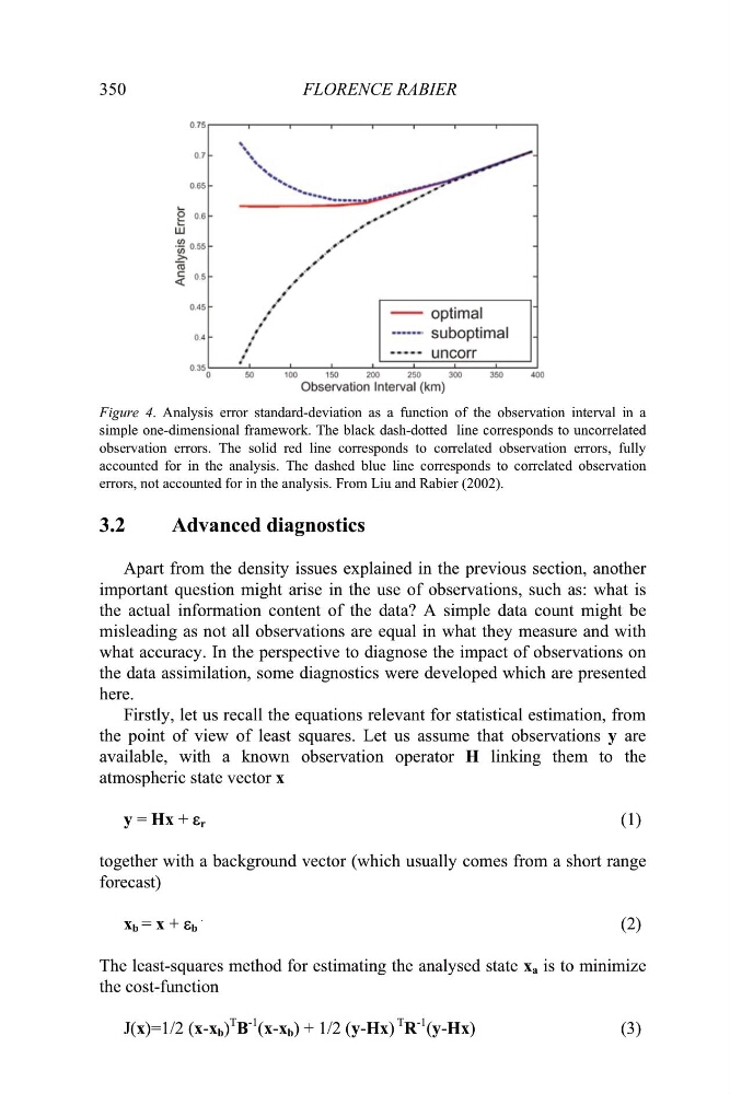
Figure 4. Analysis error standard-deviation as a function of the observation interval in a
simple one-dimensional framework. The black dash-dotted line corresponds to uncorrelated
observation errors. The solid red line corresponds to correlated observation errors, fully
accounted for in the analysis. The dashed blue line corresponds to correlated observation
errors, not accounted for in the analysis. From Liu and Rabier (2002).
3.2
Advanced diagnostics
Apart from the density issues explained in the previous section, another
important question might arise in the use of observations, such as: what is
the actual information content of the data? A simple data count might be
misleading as not all observations are equal in what they measure and with
what accuracy. In the perspective to diagnose the impact of observations on
the data assimilation, some diagnostics were developed which are presented
here.
Firstly, let us recall the equations relevant for statistical estimation, from
the point of view of least squares. Let us assume that observations y are
available, with a known observation operator H linking them to the
atmospheric state vector x
y = Hx + H r
(1)
together with a background vector (which usually comes from a short range
forecast)
x b = x + H b
.
(2)
The least-squares method for estimating the analysed state x a is to minimize
the cost-function
J(x)=1/2 (x-x b )
T
B
-1 (x-x b ) + 1/2 (y-Hx)
T
R
-1 (y-Hx)
(3)
FLORENCE RABIER
Figure 4. Analysis error standard-deviation as a function of the observation interval in a
simple one-dimensional framework. The black dash-dotted line corresponds to uncorrelated
observation errors. The solid red line corresponds to correlated observation errors, fully
accounted for in the analysis. The dashed blue line corresponds to correlated observation
errors, not accounted for in the analysis. From Liu and Rabier (2002).
3.2
Advanced diagnostics
Apart from the density issues explained in the previous section, another
important question might arise in the use of observations, such as: what is
the actual information content of the data? A simple data count might be
misleading as not all observations are equal in what they measure and with
what accuracy. In the perspective to diagnose the impact of observations on
the data assimilation, some diagnostics were developed which are presented
here.
Firstly, let us recall the equations relevant for statistical estimation, from
the point of view of least squares. Let us assume that observations y are
available, with a known observation operator H linking them to the
atmospheric state vector x
y = Hx + H r
(1)
together with a background vector (which usually comes from a short range
forecast)
x b = x + H b
.
(2)
The least-squares method for estimating the analysed state x a is to minimize
the cost-function
J(x)=1/2 (x-x b )
T
B
-1 (x-x b ) + 1/2 (y-Hx)
T
R
-1 (y-Hx)
(3)