

ICHIRO FUKUMORI
318
measurements. Moreover, most data assimilation schemes incorporate
approximations and/or simplifications that dictate what is being solved and
how the results could be utilized. For instance, because of data increments,
budgets of heat and other properties cannot be closed in a physically
consistent manner for many sequential data assimilation estimates while for
other estimates budgets can be closed. Understanding what is being solved
and how it is done so are fundamental to utilizing data assimilated estimates
and to devising means of improving them further.
The nature of the data assimilation problem and some of its solutions are
reviewed to clarify these underlying properties and to elucidate their
implications. The data assimilation problem is mathematically identified in
Section 2. In Section 3, the Kalman filter and Rauch-Tung-Striebel
smoother are compared in the context of a least-squares solution to this
mathematical problem. The nature of data and model errors that are utilized
implementing these solutions are described in Section 5, using examples
from the near real-time data assimilation system of the Consortium for
al. 2002.) The discussion is summarized in Section 6.
2. Data assimilation as an inverse problem
Mathematically, data assimilation can be identified as an inverse
problem; the state of a dynamic system (model), , and its controls, u, (nonstate variables of the model) are estimated given a set of observations,
x
y ,
and a model; e.g.,
1
1
1
2
1
1
t
t
t
t
t
t
t
t
t
t
§
·
¨
¸
¨
¸
¨
¸
¨
¸ |
¨
¸
¨
¸
¨
¸
¨
¸
¨
¸
¨
¸
©
¹
Hx
y
Hx
y
x
Ax Gu
0
x
Ax
Gu
0
§
·
¨
¸
¨
¸
¨
¸
¨
¸
¨
¸
¨
¸
¨
¸
¨
¸
¨
¸
¨
¸
©
¹
(1)
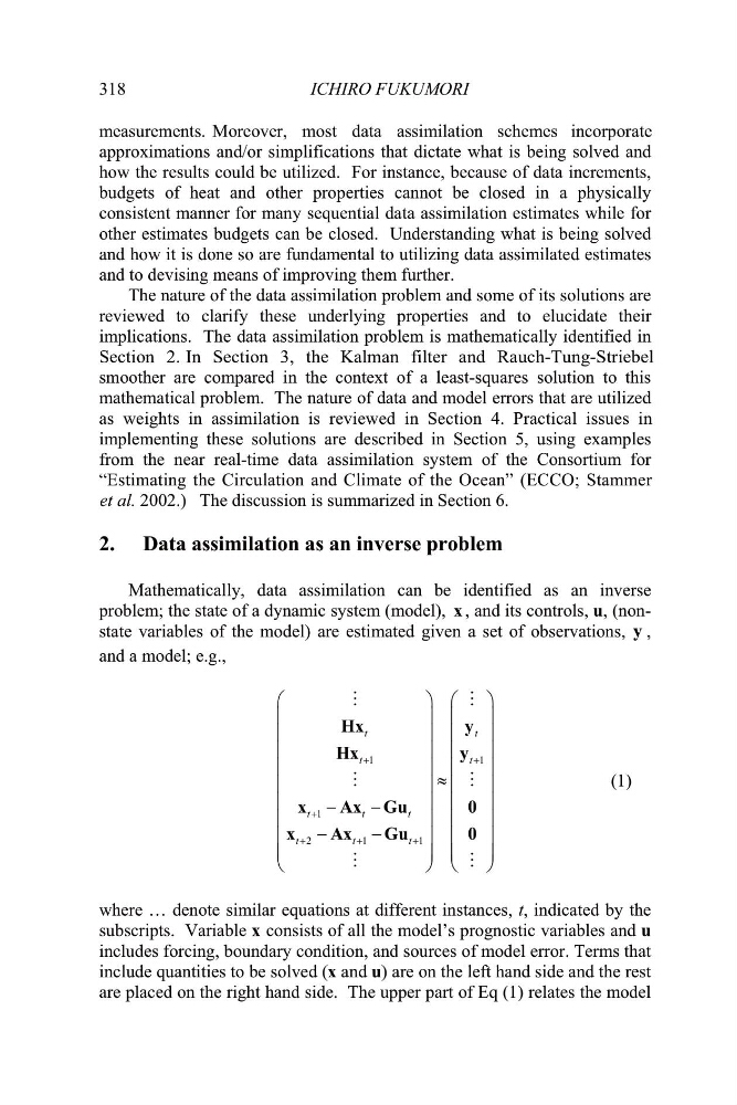
where } denote similar equations at different instances, t, indicated by the
subscripts. Variable x consists of all the model’s prognostic variables and u
includes forcing, boundary condition, and sources of model error. Terms that
include quantities to be solved (x and u) are on the left hand side and the rest
are placed on the right hand side. The upper part of Eq (1) relates the model
as weights in assimilation is reviewed in Section 4. Practical issues in
“Estimating the Circulation and Climate of the Ocean” (ECCO; Stammer
et
318
measurements. Moreover, most data assimilation schemes incorporate
approximations and/or simplifications that dictate what is being solved and
how the results could be utilized. For instance, because of data increments,
budgets of heat and other properties cannot be closed in a physically
consistent manner for many sequential data assimilation estimates while for
other estimates budgets can be closed. Understanding what is being solved
and how it is done so are fundamental to utilizing data assimilated estimates
and to devising means of improving them further.
The nature of the data assimilation problem and some of its solutions are
reviewed to clarify these underlying properties and to elucidate their
implications. The data assimilation problem is mathematically identified in
Section 2. In Section 3, the Kalman filter and Rauch-Tung-Striebel
smoother are compared in the context of a least-squares solution to this
mathematical problem. The nature of data and model errors that are utilized
implementing these solutions are described in Section 5, using examples
from the near real-time data assimilation system of the Consortium for
al. 2002.) The discussion is summarized in Section 6.
2. Data assimilation as an inverse problem
Mathematically, data assimilation can be identified as an inverse
problem; the state of a dynamic system (model), , and its controls, u, (nonstate variables of the model) are estimated given a set of observations,
x
y ,
and a model; e.g.,
1
1
1
2
1
1
t
t
t
t
t
t
t
t
t
t
§
·
¨
¸
¨
¸
¨
¸
¨
¸ |
¨
¸
¨
¸
¨
¸
¨
¸
¨
¸
¨
¸
©
¹
Hx
y
Hx
y
x
Ax Gu
0
x
Ax
Gu
0
§
·
¨
¸
¨
¸
¨
¸
¨
¸
¨
¸
¨
¸
¨
¸
¨
¸
¨
¸
¨
¸
©
¹
(1)
where } denote similar equations at different instances, t, indicated by the
subscripts. Variable x consists of all the model’s prognostic variables and u
includes forcing, boundary condition, and sources of model error. Terms that
include quantities to be solved (x and u) are on the left hand side and the rest
are placed on the right hand side. The upper part of Eq (1) relates the model
as weights in assimilation is reviewed in Section 4. Practical issues in
“Estimating the Circulation and Climate of the Ocean” (ECCO; Stammer
et