

232
WILLIAM B. LARGE
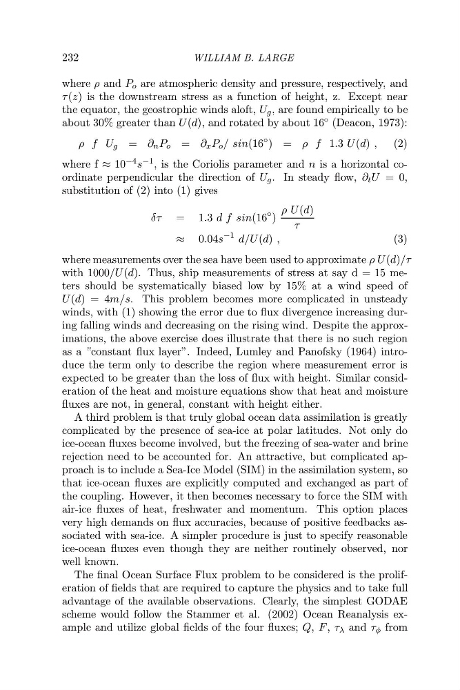
where ρ and P o are atmospheric density and pressure, respectively, and
τ (z) is the downstream stress as a function of height, z. Except near
the equator, the geostrophic winds aloft, U g , are found empirically to be
about 30% greater than U (d), and rotated by about 16 ◦ (Deacon, 1973):
ρ f U g = ∂ n P o = ∂ x P o / sin(16
◦ ) = ρ f 1.3 U (d) , (2)
where f ≈ 10 −4 s −1 , is the Coriolis parameter and n is a horizontal coordinate perpendicular the direction of U g . In steady flow, ∂ t U = 0,
substitution of (2) into (1) gives
δτ = 1.3 d f sin(16
◦ )
ρ U(d)
τ
≈ 0.04s
−1 d/U (d) ,
(3)
where measurements over the sea have been used to approximate ρ U(d)/τ
with 1000/U (d). Thus, ship measurements of stress at say d = 15 meters should be systematically biased low by 15% at a wind speed of
U (d) = 4m/s. This problem becomes more complicated in unsteady
winds, with (1) showing the error due to flux divergence increasing during falling winds and decreasing on the rising wind. Despite the approximations, the above exercise does illustrate that there is no such region
as a ”constant flux layer”. Indeed, Lumley and Panofsky (1964) introduce the term only to describe the region where measurement error is
expected to be greater than the loss of flux with height. Similar consideration of the heat and moisture equations show that heat and moisture
fluxes are not, in general, constant with height either.
A third problem is that truly global ocean data assimilation is greatly
complicated by the presence of sea-ice at polar latitudes. Not only do
ice-ocean fluxes become involved, but the freezing of sea-water and brine
rejection need to be accounted for. An attractive, but complicated approach is to include a Sea-Ice Model (SIM) in the assimilation system, so
that ice-ocean fluxes are explicitly computed and exchanged as part of
the coupling. However, it then becomes necessary to force the SIM with
air-ice fluxes of heat, freshwater and momentum. This option places
very high demands on flux accuracies, because of positive feedbacks associated with sea-ice. A simpler procedure is just to specify reasonable
ice-ocean fluxes even though they are neither routinely observed, nor
well known.
The final Ocean Surface Flux problem to be considered is the proliferation of fields that are required to capture the physics and to take full
advantage of the available observations. Clearly, the simplest GODAE
scheme would follow the Stammer et al. (2002) Ocean Reanalysis example and utilize global fields of the four fluxes; Q, F , τ λ and τ φ from
WILLIAM B. LARGE
where ρ and P o are atmospheric density and pressure, respectively, and
τ (z) is the downstream stress as a function of height, z. Except near
the equator, the geostrophic winds aloft, U g , are found empirically to be
about 30% greater than U (d), and rotated by about 16 ◦ (Deacon, 1973):
ρ f U g = ∂ n P o = ∂ x P o / sin(16
◦ ) = ρ f 1.3 U (d) , (2)
where f ≈ 10 −4 s −1 , is the Coriolis parameter and n is a horizontal coordinate perpendicular the direction of U g . In steady flow, ∂ t U = 0,
substitution of (2) into (1) gives
δτ = 1.3 d f sin(16
◦ )
ρ U(d)
τ
≈ 0.04s
−1 d/U (d) ,
(3)
where measurements over the sea have been used to approximate ρ U(d)/τ
with 1000/U (d). Thus, ship measurements of stress at say d = 15 meters should be systematically biased low by 15% at a wind speed of
U (d) = 4m/s. This problem becomes more complicated in unsteady
winds, with (1) showing the error due to flux divergence increasing during falling winds and decreasing on the rising wind. Despite the approximations, the above exercise does illustrate that there is no such region
as a ”constant flux layer”. Indeed, Lumley and Panofsky (1964) introduce the term only to describe the region where measurement error is
expected to be greater than the loss of flux with height. Similar consideration of the heat and moisture equations show that heat and moisture
fluxes are not, in general, constant with height either.
A third problem is that truly global ocean data assimilation is greatly
complicated by the presence of sea-ice at polar latitudes. Not only do
ice-ocean fluxes become involved, but the freezing of sea-water and brine
rejection need to be accounted for. An attractive, but complicated approach is to include a Sea-Ice Model (SIM) in the assimilation system, so
that ice-ocean fluxes are explicitly computed and exchanged as part of
the coupling. However, it then becomes necessary to force the SIM with
air-ice fluxes of heat, freshwater and momentum. This option places
very high demands on flux accuracies, because of positive feedbacks associated with sea-ice. A simpler procedure is just to specify reasonable
ice-ocean fluxes even though they are neither routinely observed, nor
well known.
The final Ocean Surface Flux problem to be considered is the proliferation of fields that are required to capture the physics and to take full
advantage of the available observations. Clearly, the simplest GODAE
scheme would follow the Stammer et al. (2002) Ocean Reanalysis example and utilize global fields of the four fluxes; Q, F , τ λ and τ φ from