

142
ERIC BLAYO AND LAURENT DEBREU
the external model, which is generally available in a configuration fully
overlapping Ω loc , must be modified to add an open boundary. Moreover,
once this is done, one has to find and implement an algorithm ensuring that the solutions u ext and u loc will satisfy the desired regularity
conditions through Γ.
These difficulties explain that this problem has never been addressed
before in ocean and atmosphere modelling. This can be done however
within the mathematical framework of domain decomposition methods.
These methods have been intensively studied and developed since the
end of the eighties due to the advent of parallel computers. Without going into details, let us present the global-in-time non-overlapping
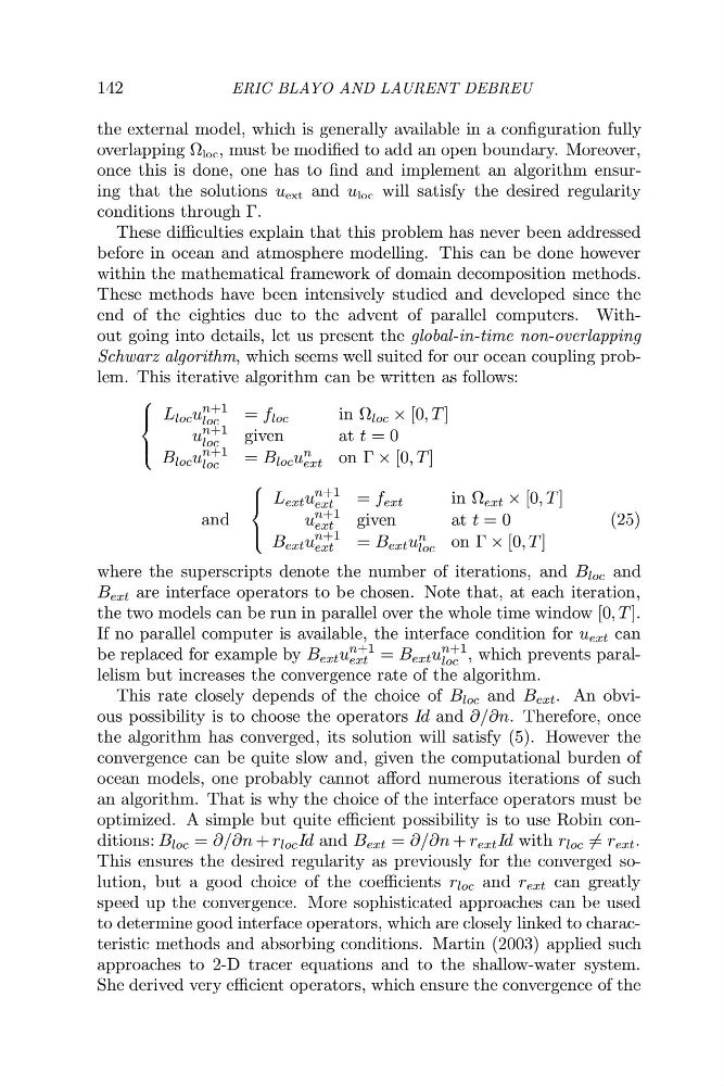
Schwarz algorithm, which seems well suited for our ocean coupling problem. This iterative algorithm can be written as follows:
⎧
⎪ ⎨
⎪ ⎩
L loc u
n+1
loc
= f loc
in Ω loc × [0, T ]
u
n+1
loc
given
at t = 0
B loc u
n+1
loc
= B loc u n
ext on Γ × [0, T ]
and
⎧
⎪ ⎨
⎪ ⎩
L ext u
n+1
ext
= f ext
in Ω ext × [0, T ]
u
n+1
ext
given
at t = 0
B ext u
n+1
ext
= B ext u n
loc on Γ × [0, T ]
(25)
where the superscripts denote the number of iterations, and B loc and
B ext are interface operators to be chosen. Note that, at each iteration,
the two models can be run in parallel over the whole time window [0, T ].
If no parallel computer is available, the interface condition for u ext can
be replaced for example by B ext u
n+1
ext = B ext u
n+1
loc , which prevents parallelism but increases the convergence rate of the algorithm.
This rate closely depends of the choice of B loc and B ext . An obvious possibility is to choose the operators Id and ∂/∂n. Therefore, once
the algorithm has converged, its solution will satisfy (5). However the
convergence can be quite slow and, given the computational burden of
ocean models, one probably cannot afford numerous iterations of such
an algorithm. That is why the choice of the interface operators must be
optimized. A simple but quite efficient possibility is to use Robin conditions: B loc = ∂/∂n + r loc Id and B ext = ∂/∂n + r ext Id with r loc = r ext .
This ensures the desired regularity as previously for the converged solution, but a good choice of the coefficients r loc and r ext can greatly
speed up the convergence. More sophisticated approaches can be used
to determine good interface operators, which are closely linked to characteristic methods and absorbing conditions. Martin (2003) applied such
approaches to 2-D tracer equations and to the shallow-water system.
She derived very efficient operators, which ensure the convergence of the
ERIC BLAYO AND LAURENT DEBREU
the external model, which is generally available in a configuration fully
overlapping Ω loc , must be modified to add an open boundary. Moreover,
once this is done, one has to find and implement an algorithm ensuring that the solutions u ext and u loc will satisfy the desired regularity
conditions through Γ.
These difficulties explain that this problem has never been addressed
before in ocean and atmosphere modelling. This can be done however
within the mathematical framework of domain decomposition methods.
These methods have been intensively studied and developed since the
end of the eighties due to the advent of parallel computers. Without going into details, let us present the global-in-time non-overlapping
Schwarz algorithm, which seems well suited for our ocean coupling problem. This iterative algorithm can be written as follows:
⎧
⎪ ⎨
⎪ ⎩
L loc u
n+1
loc
= f loc
in Ω loc × [0, T ]
u
n+1
loc
given
at t = 0
B loc u
n+1
loc
= B loc u n
ext on Γ × [0, T ]
and
⎧
⎪ ⎨
⎪ ⎩
L ext u
n+1
ext
= f ext
in Ω ext × [0, T ]
u
n+1
ext
given
at t = 0
B ext u
n+1
ext
= B ext u n
loc on Γ × [0, T ]
(25)
where the superscripts denote the number of iterations, and B loc and
B ext are interface operators to be chosen. Note that, at each iteration,
the two models can be run in parallel over the whole time window [0, T ].
If no parallel computer is available, the interface condition for u ext can
be replaced for example by B ext u
n+1
ext = B ext u
n+1
loc , which prevents parallelism but increases the convergence rate of the algorithm.
This rate closely depends of the choice of B loc and B ext . An obvious possibility is to choose the operators Id and ∂/∂n. Therefore, once
the algorithm has converged, its solution will satisfy (5). However the
convergence can be quite slow and, given the computational burden of
ocean models, one probably cannot afford numerous iterations of such
an algorithm. That is why the choice of the interface operators must be
optimized. A simple but quite efficient possibility is to use Robin conditions: B loc = ∂/∂n + r loc Id and B ext = ∂/∂n + r ext Id with r loc = r ext .
This ensures the desired regularity as previously for the converged solution, but a good choice of the coefficients r loc and r ext can greatly
speed up the convergence. More sophisticated approaches can be used
to determine good interface operators, which are closely linked to characteristic methods and absorbing conditions. Martin (2003) applied such
approaches to 2-D tracer equations and to the shallow-water system.
She derived very efficient operators, which ensure the convergence of the