

3.19 Exercise 11: Double-Diffusive Instability
75
where ρ
is density anomaly, the thermal expansion coefficient is set to α = 2.5 ×
10
−4 K
−1 , and the salinity coefficient is set to β = 8×10
−4 . The advection-diffusion
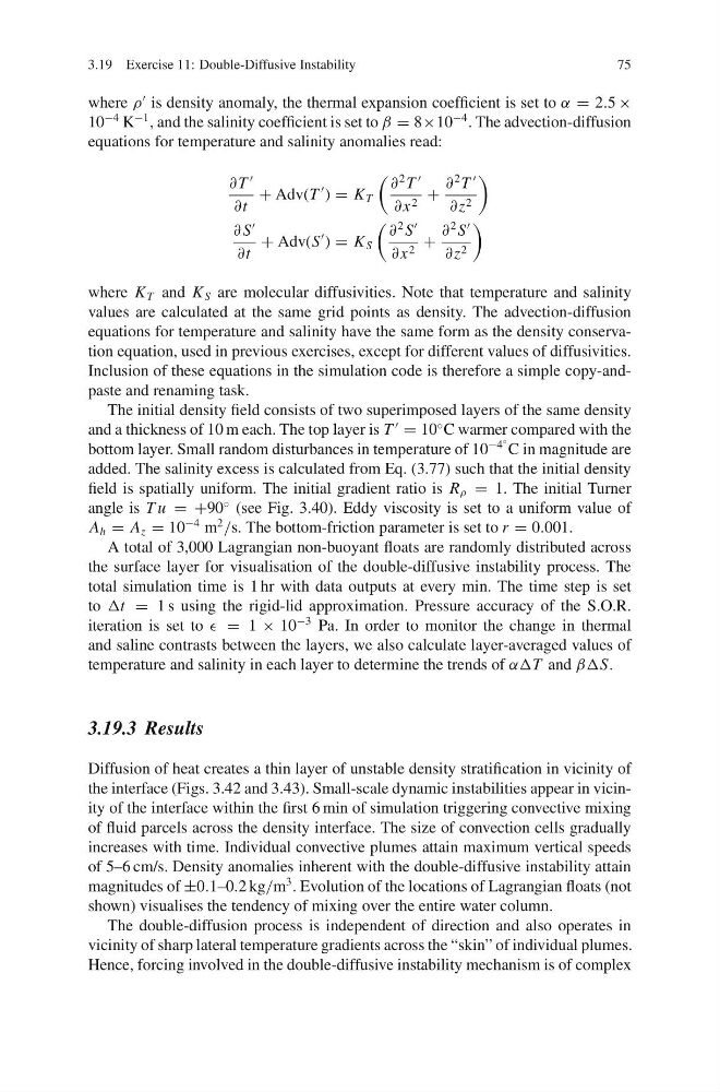
equations for temperature and salinity anomalies read:
∂ T
∂t
+ Adv(T
) = K T
∂
2 T
∂ x 2 +
∂
2 T
∂z 2
∂ S
∂t
+ Adv(S
) = K S
∂
2 S
∂ x 2 +
∂
2 S
∂z 2
where K T and K S are molecular diffusivities. Note that temperature and salinity
values are calculated at the same grid points as density. The advection-diffusion
equations for temperature and salinity have the same form as the density conservation equation, used in previous exercises, except for different values of diffusivities.
Inclusion of these equations in the simulation code is therefore a simple copy-andpaste and renaming task.
The initial density field consists of two superimposed layers of the same density
and a thickness of 10 m each. The top layer is T
= 10
◦ C warmer compared with the
bottom layer. Small random disturbances in temperature of 10
−4
◦ C in magnitude are
added. The salinity excess is calculated from Eq. (3.77) such that the initial density
field is spatially uniform. The initial gradient ratio is R ρ = 1. The initial Turner
angle is T u = +90
◦ (see Fig. 3.40). Eddy viscosity is set to a uniform value of
A h = A z = 10
−4 m
2
/s. The bottom-friction parameter is set to r = 0.001.
A total of 3,000 Lagrangian non-buoyant floats are randomly distributed across
the surface layer for visualisation of the double-diffusive instability process. The
total simulation time is 1 hr with data outputs at every min. The time step is set
to Δt = 1 s using the rigid-lid approximation. Pressure accuracy of the S.O.R.
iteration is set to = 1 × 10
−3 Pa. In order to monitor the change in thermal
and saline contrasts between the layers, we also calculate layer-averaged values of
temperature and salinity in each layer to determine the trends of αΔT and βΔS.
3.19.3 Results
Diffusion of heat creates a thin layer of unstable density stratification in vicinity of
the interface (Figs. 3.42 and 3.43). Small-scale dynamic instabilities appear in vicinity of the interface within the first 6 min of simulation triggering convective mixing
of fluid parcels across the density interface. The size of convection cells gradually
increases with time. Individual convective plumes attain maximum vertical speeds
of 5–6 cm/s. Density anomalies inherent with the double-diffusive instability attain
magnitudes of ±0.1–0.2 kg/m
3 . Evolution of the locations of Lagrangian floats (not
shown) visualises the tendency of mixing over the entire water column.
The double-diffusion process is independent of direction and also operates in
vicinity of sharp lateral temperature gradients across the “skin” of individual plumes.
Hence, forcing involved in the double-diffusive instability mechanism is of complex
75
where ρ
is density anomaly, the thermal expansion coefficient is set to α = 2.5 ×
10
−4 K
−1 , and the salinity coefficient is set to β = 8×10
−4 . The advection-diffusion
equations for temperature and salinity anomalies read:
∂ T
∂t
+ Adv(T
) = K T
∂
2 T
∂ x 2 +
∂
2 T
∂z 2
∂ S
∂t
+ Adv(S
) = K S
∂
2 S
∂ x 2 +
∂
2 S
∂z 2
where K T and K S are molecular diffusivities. Note that temperature and salinity
values are calculated at the same grid points as density. The advection-diffusion
equations for temperature and salinity have the same form as the density conservation equation, used in previous exercises, except for different values of diffusivities.
Inclusion of these equations in the simulation code is therefore a simple copy-andpaste and renaming task.
The initial density field consists of two superimposed layers of the same density
and a thickness of 10 m each. The top layer is T
= 10
◦ C warmer compared with the
bottom layer. Small random disturbances in temperature of 10
−4
◦ C in magnitude are
added. The salinity excess is calculated from Eq. (3.77) such that the initial density
field is spatially uniform. The initial gradient ratio is R ρ = 1. The initial Turner
angle is T u = +90
◦ (see Fig. 3.40). Eddy viscosity is set to a uniform value of
A h = A z = 10
−4 m
2
/s. The bottom-friction parameter is set to r = 0.001.
A total of 3,000 Lagrangian non-buoyant floats are randomly distributed across
the surface layer for visualisation of the double-diffusive instability process. The
total simulation time is 1 hr with data outputs at every min. The time step is set
to Δt = 1 s using the rigid-lid approximation. Pressure accuracy of the S.O.R.
iteration is set to = 1 × 10
−3 Pa. In order to monitor the change in thermal
and saline contrasts between the layers, we also calculate layer-averaged values of
temperature and salinity in each layer to determine the trends of αΔT and βΔS.
3.19.3 Results
Diffusion of heat creates a thin layer of unstable density stratification in vicinity of
the interface (Figs. 3.42 and 3.43). Small-scale dynamic instabilities appear in vicinity of the interface within the first 6 min of simulation triggering convective mixing
of fluid parcels across the density interface. The size of convection cells gradually
increases with time. Individual convective plumes attain maximum vertical speeds
of 5–6 cm/s. Density anomalies inherent with the double-diffusive instability attain
magnitudes of ±0.1–0.2 kg/m
3 . Evolution of the locations of Lagrangian floats (not
shown) visualises the tendency of mixing over the entire water column.
The double-diffusion process is independent of direction and also operates in
vicinity of sharp lateral temperature gradients across the “skin” of individual plumes.
Hence, forcing involved in the double-diffusive instability mechanism is of complex