

3.17 Exercise 10: Slope Convection near the Shore
69
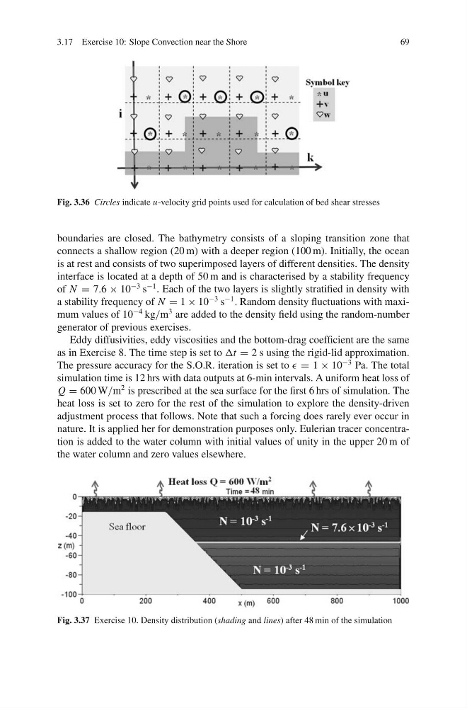
Fig. 3.36 Circles indicate u-velocity grid points used for calculation of bed shear stresses
boundaries are closed. The bathymetry consists of a sloping transition zone that
connects a shallow region (20 m) with a deeper region (100 m). Initially, the ocean
is at rest and consists of two superimposed layers of different densities. The density
interface is located at a depth of 50 m and is characterised by a stability frequency
of N = 7.6 × 10
−3 s
−1 . Each of the two layers is slightly stratified in density with
a stability frequency of N = 1 × 10
−3 s
−1 . Random density fluctuations with maximum values of 10
−4 kg/m
3 are added to the density field using the random-number
generator of previous exercises.
Eddy diffusivities, eddy viscosities and the bottom-drag coefficient are the same
as in Exercise 8. The time step is set to Δt = 2 s using the rigid-lid approximation.
The pressure accuracy for the S.O.R. iteration is set to = 1 × 10
−3 Pa. The total
simulation time is 12 hrs with data outputs at 6-min intervals. A uniform heat loss of
Q = 600 W/m
2 is prescribed at the sea surface for the first 6 hrs of simulation. The
heat loss is set to zero for the rest of the simulation to explore the density-driven
adjustment process that follows. Note that such a forcing does rarely ever occur in
nature. It is applied her for demonstration purposes only. Eulerian tracer concentration is added to the water column with initial values of unity in the upper 20 m of
the water column and zero values elsewhere.
Fig. 3.37 Exercise 10. Density distribution (shading and lines) after 48 min of the simulation
69
Fig. 3.36 Circles indicate u-velocity grid points used for calculation of bed shear stresses
boundaries are closed. The bathymetry consists of a sloping transition zone that
connects a shallow region (20 m) with a deeper region (100 m). Initially, the ocean
is at rest and consists of two superimposed layers of different densities. The density
interface is located at a depth of 50 m and is characterised by a stability frequency
of N = 7.6 × 10
−3 s
−1 . Each of the two layers is slightly stratified in density with
a stability frequency of N = 1 × 10
−3 s
−1 . Random density fluctuations with maximum values of 10
−4 kg/m
3 are added to the density field using the random-number
generator of previous exercises.
Eddy diffusivities, eddy viscosities and the bottom-drag coefficient are the same
as in Exercise 8. The time step is set to Δt = 2 s using the rigid-lid approximation.
The pressure accuracy for the S.O.R. iteration is set to = 1 × 10
−3 Pa. The total
simulation time is 12 hrs with data outputs at 6-min intervals. A uniform heat loss of
Q = 600 W/m
2 is prescribed at the sea surface for the first 6 hrs of simulation. The
heat loss is set to zero for the rest of the simulation to explore the density-driven
adjustment process that follows. Note that such a forcing does rarely ever occur in
nature. It is applied her for demonstration purposes only. Eulerian tracer concentration is added to the water column with initial values of unity in the upper 20 m of
the water column and zero values elsewhere.
Fig. 3.37 Exercise 10. Density distribution (shading and lines) after 48 min of the simulation