

52
3 Basics of Nonhydrostatic Modelling
3.11.4 Results
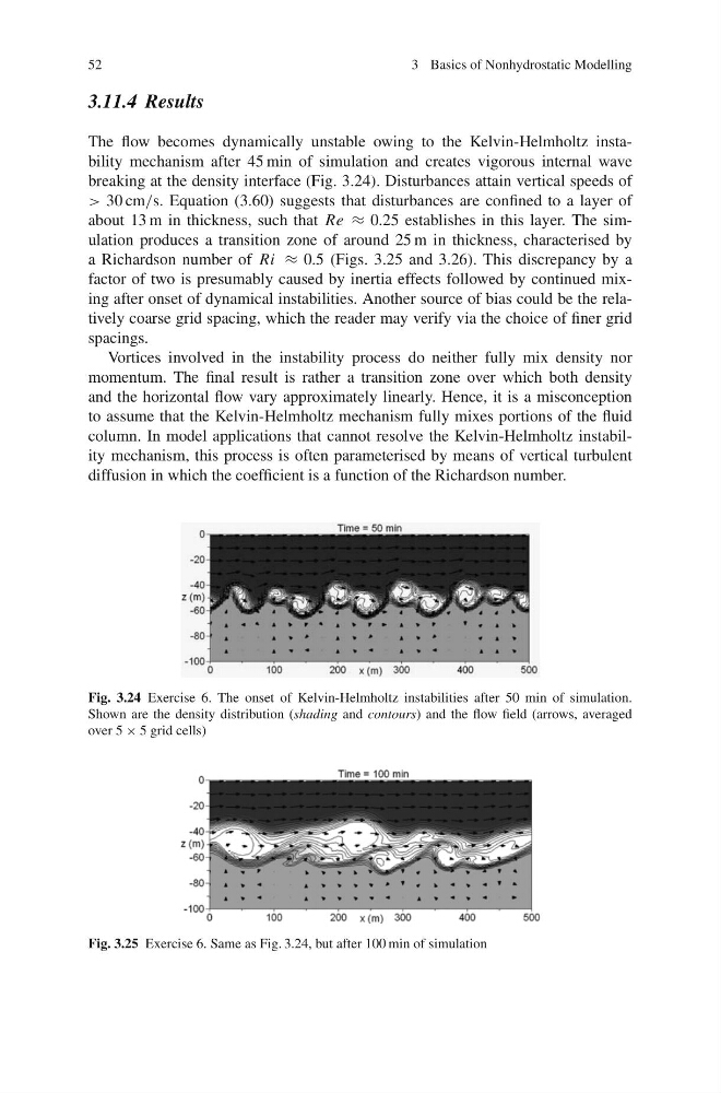
The flow becomes dynamically unstable owing to the Kelvin-Helmholtz instability mechanism after 45 min of simulation and creates vigorous internal wave
breaking at the density interface (Fig. 3.24). Disturbances attain vertical speeds of
> 30 cm/s. Equation (3.60) suggests that disturbances are confined to a layer of
about 13 m in thickness, such that Re ≈ 0.25 establishes in this layer. The simulation produces a transition zone of around 25 m in thickness, characterised by
a Richardson number of Ri ≈ 0.5 (Figs. 3.25 and 3.26). This discrepancy by a
factor of two is presumably caused by inertia effects followed by continued mixing after onset of dynamical instabilities. Another source of bias could be the relatively coarse grid spacing, which the reader may verify via the choice of finer grid
spacings.
Vortices involved in the instability process do neither fully mix density nor
momentum. The final result is rather a transition zone over which both density
and the horizontal flow vary approximately linearly. Hence, it is a misconception
to assume that the Kelvin-Helmholtz mechanism fully mixes portions of the fluid
column. In model applications that cannot resolve the Kelvin-Helmholtz instability mechanism, this process is often parameterised by means of vertical turbulent
diffusion in which the coefficient is a function of the Richardson number.
Fig. 3.24 Exercise 6. The onset of Kelvin-Helmholtz instabilities after 50 min of simulation.
Shown are the density distribution (shading and contours) and the flow field (arrows, averaged
over 5 × 5 grid cells)
Fig. 3.25 Exercise 6. Same as Fig. 3.24, but after 100 min of simulation
3 Basics of Nonhydrostatic Modelling
3.11.4 Results
The flow becomes dynamically unstable owing to the Kelvin-Helmholtz instability mechanism after 45 min of simulation and creates vigorous internal wave
breaking at the density interface (Fig. 3.24). Disturbances attain vertical speeds of
> 30 cm/s. Equation (3.60) suggests that disturbances are confined to a layer of
about 13 m in thickness, such that Re ≈ 0.25 establishes in this layer. The simulation produces a transition zone of around 25 m in thickness, characterised by
a Richardson number of Ri ≈ 0.5 (Figs. 3.25 and 3.26). This discrepancy by a
factor of two is presumably caused by inertia effects followed by continued mixing after onset of dynamical instabilities. Another source of bias could be the relatively coarse grid spacing, which the reader may verify via the choice of finer grid
spacings.
Vortices involved in the instability process do neither fully mix density nor
momentum. The final result is rather a transition zone over which both density
and the horizontal flow vary approximately linearly. Hence, it is a misconception
to assume that the Kelvin-Helmholtz mechanism fully mixes portions of the fluid
column. In model applications that cannot resolve the Kelvin-Helmholtz instability mechanism, this process is often parameterised by means of vertical turbulent
diffusion in which the coefficient is a function of the Richardson number.
Fig. 3.24 Exercise 6. The onset of Kelvin-Helmholtz instabilities after 50 min of simulation.
Shown are the density distribution (shading and contours) and the flow field (arrows, averaged
over 5 × 5 grid cells)
Fig. 3.25 Exercise 6. Same as Fig. 3.24, but after 100 min of simulation