

3.6 Inclusion of Variable Density
37
The temporal change of B can be discretised using a simple time-forward iteration. The treatment of the remaining term is described in the following for the
x-direction. Analog recipes apply for the z-direction. The general approach is to
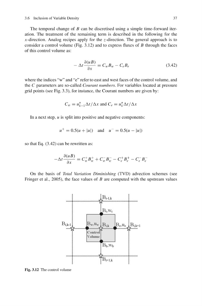
consider a control volume (Fig. 3.12) and to express fluxes of B through the faces
of this control volume as:
− Δt
∂(u B)
∂ x
= C w B w − C e B e
(3.42)
where the indices “w” and “e” refer to east and west faces of the control volume, and
the C parameters are so-called Courant numbers. For variables located at pressure
grid points (see Fig. 3.3), for instance, the Courant numbers are given by:
C w = u
n
k−1 Δt/Δx and C e = u
n
k Δt/Δx
In a next step, u is split into positive and negative components:
u
+
= 0.5(u + |u|) and u
−
= 0.5(u − |u|)
so that Eq. (3.42) can be rewritten as:
−Δt
∂(u B)
∂ x
= C
+
w B
+
w + C
−
w B
−
w − C
+
e B
+
e − C
−
e B
−
e
On the basis of Total Variation Diminishing (TVD) advection schemes (see
Fringer et al., 2005), the face values of B are computed with the upstream values
Fig. 3.12 The control volume
37
The temporal change of B can be discretised using a simple time-forward iteration. The treatment of the remaining term is described in the following for the
x-direction. Analog recipes apply for the z-direction. The general approach is to
consider a control volume (Fig. 3.12) and to express fluxes of B through the faces
of this control volume as:
− Δt
∂(u B)
∂ x
= C w B w − C e B e
(3.42)
where the indices “w” and “e” refer to east and west faces of the control volume, and
the C parameters are so-called Courant numbers. For variables located at pressure
grid points (see Fig. 3.3), for instance, the Courant numbers are given by:
C w = u
n
k−1 Δt/Δx and C e = u
n
k Δt/Δx
In a next step, u is split into positive and negative components:
u
+
= 0.5(u + |u|) and u
−
= 0.5(u − |u|)
so that Eq. (3.42) can be rewritten as:
−Δt
∂(u B)
∂ x
= C
+
w B
+
w + C
−
w B
−
w − C
+
e B
+
e − C
−
e B
−
e
On the basis of Total Variation Diminishing (TVD) advection schemes (see
Fringer et al., 2005), the face values of B are computed with the upstream values
Fig. 3.12 The control volume