

30
3 Basics of Nonhydrostatic Modelling
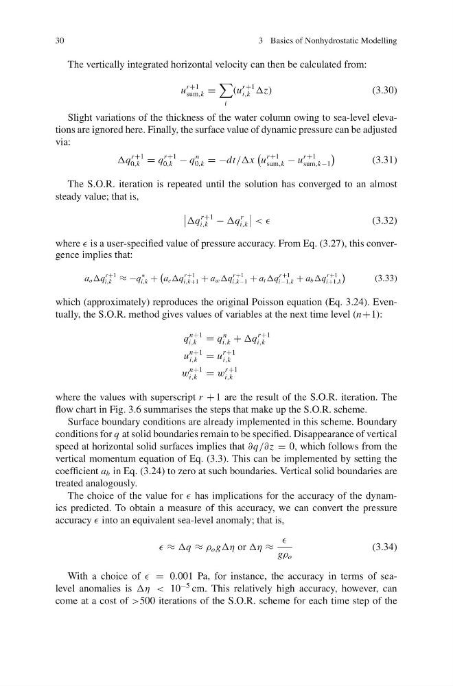
The vertically integrated horizontal velocity can then be calculated from:
u
r+1
sum,k =
i
(u
r+1
i,k Δz)
(3.30)
Slight variations of the thickness of the water column owing to sea-level elevations are ignored here. Finally, the surface value of dynamic pressure can be adjusted
via:
Δq
r +1
0,k = q
r+1
0,k − q
n
0,k = −dt/Δx
u
r +1
sum,k − u
r +1
sum,k−1
(3.31)
The S.O.R. iteration is repeated until the solution has converged to an almost
steady value; that is,
Δq
r+1
i,k − Δq
r
i,k
< <
(3.32)
where is a user-specified value of pressure accuracy. From Eq. (3.27), this convergence implies that:
a o Δq
r +1
i,k ≈ −q
∗
i,k +
a e Δq
r+1
i,k+1 + a w Δq
r+1
i,k−1 + a t Δq
r+1
i−1,k + a b Δq
r+1
i+1,k
(3.33)
which (approximately) reproduces the original Poisson equation (Eq. 3.24). Eventually, the S.O.R. method gives values of variables at the next time level (n +1):
q
n+1
i,k = q
n
i,k + Δq
r+1
i,k
u
n+1
i,k = u
r+1
i,k
w
n+1
i,k = w
r+1
i,k
where the values with superscript r + 1 are the result of the S.O.R. iteration. The
flow chart in Fig. 3.6 summarises the steps that make up the S.O.R. scheme.
Surface boundary conditions are already implemented in this scheme. Boundary
conditions for q at solid boundaries remain to be specified. Disappearance of vertical
speed at horizontal solid surfaces implies that ∂q/∂z = 0, which follows from the
vertical momentum equation of Eq. (3.3). This can be implemented by setting the
coefficient a b in Eq. (3.24) to zero at such boundaries. Vertical solid boundaries are
treated analogously.
The choice of the value for has implications for the accuracy of the dynamics predicted. To obtain a measure of this accuracy, we can convert the pressure
accuracy into an equivalent sea-level anomaly; that is,
≈ Δq ≈ ρ o gΔη or Δη ≈
gρ o
(3.34)
With a choice of = 0.001 Pa, for instance, the accuracy in terms of sealevel anomalies is Δη < 10
−5 cm. This relatively high accuracy, however, can
come at a cost of >500 iterations of the S.O.R. scheme for each time step of the
3 Basics of Nonhydrostatic Modelling
The vertically integrated horizontal velocity can then be calculated from:
u
r+1
sum,k =
i
(u
r+1
i,k Δz)
(3.30)
Slight variations of the thickness of the water column owing to sea-level elevations are ignored here. Finally, the surface value of dynamic pressure can be adjusted
via:
Δq
r +1
0,k = q
r+1
0,k − q
n
0,k = −dt/Δx
u
r +1
sum,k − u
r +1
sum,k−1
(3.31)
The S.O.R. iteration is repeated until the solution has converged to an almost
steady value; that is,
Δq
r+1
i,k − Δq
r
i,k
< <
(3.32)
where is a user-specified value of pressure accuracy. From Eq. (3.27), this convergence implies that:
a o Δq
r +1
i,k ≈ −q
∗
i,k +
a e Δq
r+1
i,k+1 + a w Δq
r+1
i,k−1 + a t Δq
r+1
i−1,k + a b Δq
r+1
i+1,k
(3.33)
which (approximately) reproduces the original Poisson equation (Eq. 3.24). Eventually, the S.O.R. method gives values of variables at the next time level (n +1):
q
n+1
i,k = q
n
i,k + Δq
r+1
i,k
u
n+1
i,k = u
r+1
i,k
w
n+1
i,k = w
r+1
i,k
where the values with superscript r + 1 are the result of the S.O.R. iteration. The
flow chart in Fig. 3.6 summarises the steps that make up the S.O.R. scheme.
Surface boundary conditions are already implemented in this scheme. Boundary
conditions for q at solid boundaries remain to be specified. Disappearance of vertical
speed at horizontal solid surfaces implies that ∂q/∂z = 0, which follows from the
vertical momentum equation of Eq. (3.3). This can be implemented by setting the
coefficient a b in Eq. (3.24) to zero at such boundaries. Vertical solid boundaries are
treated analogously.
The choice of the value for has implications for the accuracy of the dynamics predicted. To obtain a measure of this accuracy, we can convert the pressure
accuracy into an equivalent sea-level anomaly; that is,
≈ Δq ≈ ρ o gΔη or Δη ≈
gρ o
(3.34)
With a choice of = 0.001 Pa, for instance, the accuracy in terms of sealevel anomalies is Δη < 10
−5 cm. This relatively high accuracy, however, can
come at a cost of >500 iterations of the S.O.R. scheme for each time step of the