

154
5 3D Level Modelling
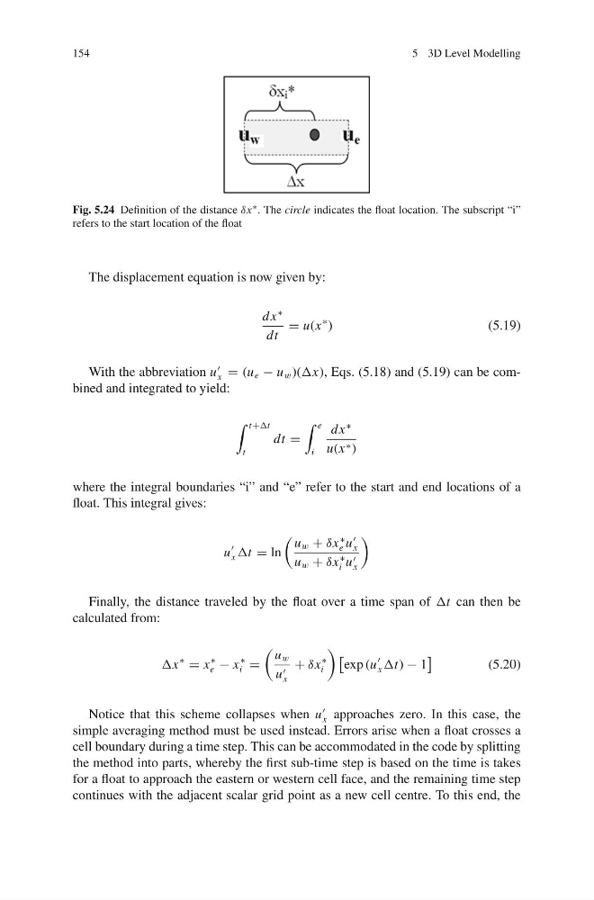
Fig. 5.24 Definition of the distance δx
∗ . The circle indicates the float location. The subscript “i”
refers to the start location of the float
The displacement equation is now given by:
dx
∗
dt
= u(x
∗ )
(5.19)
With the abbreviation u
x = (u e − u w )(Δx), Eqs. (5.18) and (5.19) can be combined and integrated to yield:
t+Δt
t
dt =
e
i
dx
∗
u(x ∗ )
where the integral boundaries “i” and “e” refer to the start and end locations of a
float. This integral gives:
u
x Δt = ln
u w + δx
∗
e u
x
u w + δx
∗
i u
x
Finally, the distance traveled by the float over a time span of Δt can then be
calculated from:
Δx
∗
= x
∗
e − x
∗
i =
u w
u
x
+ δx
∗
i
exp (u
x Δt) − 1
(5.20)
Notice that this scheme collapses when u
x approaches zero. In this case, the
simple averaging method must be used instead. Errors arise when a float crosses a
cell boundary during a time step. This can be accommodated in the code by splitting
the method into parts, whereby the first sub-time step is based on the time is takes
for a float to approach the eastern or western cell face, and the remaining time step
continues with the adjacent scalar grid point as a new cell centre. To this end, the
5 3D Level Modelling
Fig. 5.24 Definition of the distance δx
∗ . The circle indicates the float location. The subscript “i”
refers to the start location of the float
The displacement equation is now given by:
dx
∗
dt
= u(x
∗ )
(5.19)
With the abbreviation u
x = (u e − u w )(Δx), Eqs. (5.18) and (5.19) can be combined and integrated to yield:
t+Δt
t
dt =
e
i
dx
∗
u(x ∗ )
where the integral boundaries “i” and “e” refer to the start and end locations of a
float. This integral gives:
u
x Δt = ln
u w + δx
∗
e u
x
u w + δx
∗
i u
x
Finally, the distance traveled by the float over a time span of Δt can then be
calculated from:
Δx
∗
= x
∗
e − x
∗
i =
u w
u
x
+ δx
∗
i
exp (u
x Δt) − 1
(5.20)
Notice that this scheme collapses when u
x approaches zero. In this case, the
simple averaging method must be used instead. Errors arise when a float crosses a
cell boundary during a time step. This can be accommodated in the code by splitting
the method into parts, whereby the first sub-time step is based on the time is takes
for a float to approach the eastern or western cell face, and the remaining time step
continues with the adjacent scalar grid point as a new cell centre. To this end, the