

130
5 3D Level Modelling
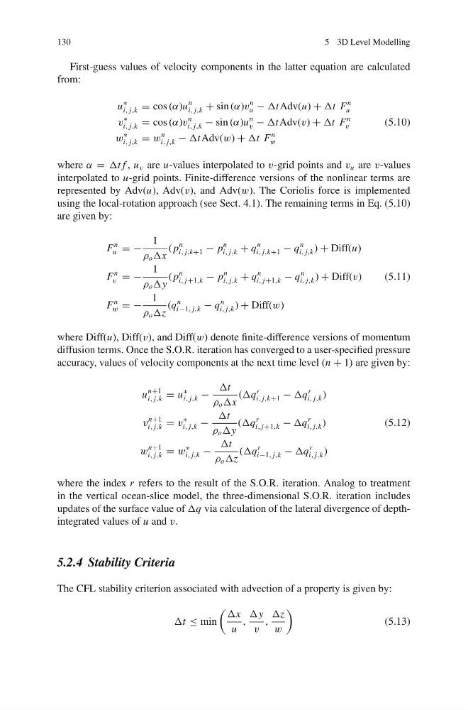
First-guess values of velocity components in the latter equation are calculated
from:
u
∗
i, j,k = cos (α)u
n
i, j,k + sin (α)v
n
u − ΔtAdv(u) + Δt F
n
u
v
∗
i, j,k = cos (α)v
n
i, j,k − sin (α)u
n
v − ΔtAdv(v) + Δt F
n
v
(5.10)
w
∗
i, j,k = w
n
i, j,k − ΔtAdv(w) + Δt F
n
w
where α = Δt f , u v are u-values interpolated to v-grid points and v u are v-values
interpolated to u-grid points. Finite-difference versions of the nonlinear terms are
represented by Adv(u), Adv(v), and Adv(w). The Coriolis force is implemented
using the local-rotation approach (see Sect. 4.1). The remaining terms in Eq. (5.10)
are given by:
F
n
u = −
1
ρ o Δx
( p
n
i, j,k+1 − p
n
i, j,k + q
n
i, j,k+1 − q
n
i, j,k ) + Diff(u)
F
n
v = −
1
ρ o Δy
( p
n
i, j+1,k − p
n
i, j,k + q
n
i, j+1,k − q
n
i, j,k ) + Diff(v)
(5.11)
F
n
w = −
1
ρ o Δz
(q
n
i−1, j,k − q
n
i, j,k ) + Diff(w)
where Diff(u), Diff(v), and Diff(w) denote finite-difference versions of momentum
diffusion terms. Once the S.O.R. iteration has converged to a user-specified pressure
accuracy, values of velocity components at the next time level (n + 1) are given by:
u
n+1
i, j,k = u
∗
i, j,k −
Δt
ρ o Δx
(Δq
r
i, j,k+1 − Δq
r
i, j,k )
v
n+1
i, j,k = v
∗
i, j,k −
Δt
ρ o Δy
(Δq
r
i, j+1,k − Δq
r
i, j,k )
(5.12)
w
n+1
i, j,k = w
∗
i, j,k −
Δt
ρ o Δz
(Δq
r
i−1, j,k − Δq
r
i, j,k )
where the index r refers to the result of the S.O.R. iteration. Analog to treatment
in the vertical ocean-slice model, the three-dimensional S.O.R. iteration includes
updates of the surface value of Δq via calculation of the lateral divergence of depthintegrated values of u and v.
5.2.4 Stability Criteria
The CFL stability criterion associated with advection of a property is given by:
Δt ≤ min
Δx
u
,
Δy
v
,
Δz
w
(5.13)
5 3D Level Modelling
First-guess values of velocity components in the latter equation are calculated
from:
u
∗
i, j,k = cos (α)u
n
i, j,k + sin (α)v
n
u − ΔtAdv(u) + Δt F
n
u
v
∗
i, j,k = cos (α)v
n
i, j,k − sin (α)u
n
v − ΔtAdv(v) + Δt F
n
v
(5.10)
w
∗
i, j,k = w
n
i, j,k − ΔtAdv(w) + Δt F
n
w
where α = Δt f , u v are u-values interpolated to v-grid points and v u are v-values
interpolated to u-grid points. Finite-difference versions of the nonlinear terms are
represented by Adv(u), Adv(v), and Adv(w). The Coriolis force is implemented
using the local-rotation approach (see Sect. 4.1). The remaining terms in Eq. (5.10)
are given by:
F
n
u = −
1
ρ o Δx
( p
n
i, j,k+1 − p
n
i, j,k + q
n
i, j,k+1 − q
n
i, j,k ) + Diff(u)
F
n
v = −
1
ρ o Δy
( p
n
i, j+1,k − p
n
i, j,k + q
n
i, j+1,k − q
n
i, j,k ) + Diff(v)
(5.11)
F
n
w = −
1
ρ o Δz
(q
n
i−1, j,k − q
n
i, j,k ) + Diff(w)
where Diff(u), Diff(v), and Diff(w) denote finite-difference versions of momentum
diffusion terms. Once the S.O.R. iteration has converged to a user-specified pressure
accuracy, values of velocity components at the next time level (n + 1) are given by:
u
n+1
i, j,k = u
∗
i, j,k −
Δt
ρ o Δx
(Δq
r
i, j,k+1 − Δq
r
i, j,k )
v
n+1
i, j,k = v
∗
i, j,k −
Δt
ρ o Δy
(Δq
r
i, j+1,k − Δq
r
i, j,k )
(5.12)
w
n+1
i, j,k = w
∗
i, j,k −
Δt
ρ o Δz
(Δq
r
i−1, j,k − Δq
r
i, j,k )
where the index r refers to the result of the S.O.R. iteration. Analog to treatment
in the vertical ocean-slice model, the three-dimensional S.O.R. iteration includes
updates of the surface value of Δq via calculation of the lateral divergence of depthintegrated values of u and v.
5.2.4 Stability Criteria
The CFL stability criterion associated with advection of a property is given by:
Δt ≤ min
Δx
u
,
Δy
v
,
Δz
w
(5.13)