

100
4 2.5D Vertical Slice Modelling
where h i is the thickness of a layer, and relative vorticity is given by:
ξ i =
∂v i
∂ x
−
∂u i
∂ y
(4.11)
In this context, the Coriolis parameter f is referred to as planetary vorticity. It is
obvious from this principle that localised water-column stretching or squeezing can
produce swift geostrophic flow disturbances.
4.1.5 Geostrophic Adjustment
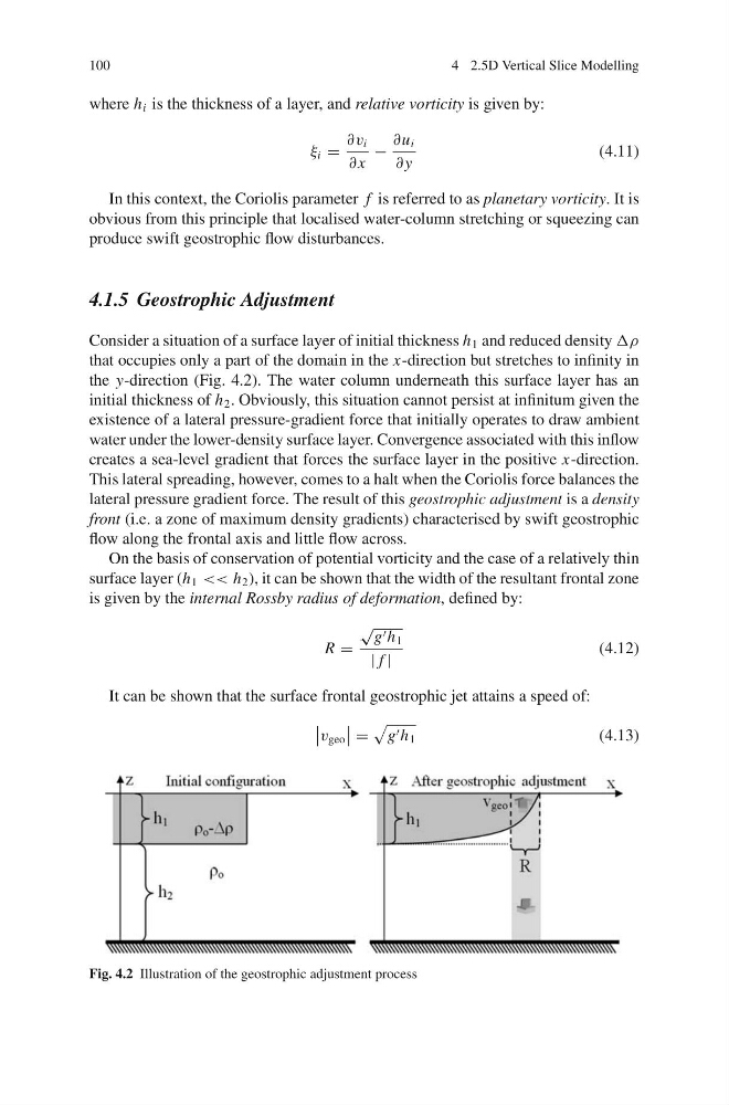
Consider a situation of a surface layer of initial thickness h 1 and reduced density Δρ
that occupies only a part of the domain in the x-direction but stretches to infinity in
the y-direction (Fig. 4.2). The water column underneath this surface layer has an
initial thickness of h 2 . Obviously, this situation cannot persist at infinitum given the
existence of a lateral pressure-gradient force that initially operates to draw ambient
water under the lower-density surface layer. Convergence associated with this inflow
creates a sea-level gradient that forces the surface layer in the positive x-direction.
This lateral spreading, however, comes to a halt when the Coriolis force balances the
lateral pressure gradient force. The result of this geostrophic adjustment is a density
front (i.e. a zone of maximum density gradients) characterised by swift geostrophic
flow along the frontal axis and little flow across.
On the basis of conservation of potential vorticity and the case of a relatively thin
surface layer (h 1 << h 2 ), it can be shown that the width of the resultant frontal zone
is given by the internal Rossby radius of deformation, defined by:
R =
√
g h 1
| f |
(4.12)
It can be shown that the surface frontal geostrophic jet attains a speed of:
v geo
=
g h 1
(4.13)
Fig. 4.2 Illustration of the geostrophic adjustment process
4 2.5D Vertical Slice Modelling
where h i is the thickness of a layer, and relative vorticity is given by:
ξ i =
∂v i
∂ x
−
∂u i
∂ y
(4.11)
In this context, the Coriolis parameter f is referred to as planetary vorticity. It is
obvious from this principle that localised water-column stretching or squeezing can
produce swift geostrophic flow disturbances.
4.1.5 Geostrophic Adjustment
Consider a situation of a surface layer of initial thickness h 1 and reduced density Δρ
that occupies only a part of the domain in the x-direction but stretches to infinity in
the y-direction (Fig. 4.2). The water column underneath this surface layer has an
initial thickness of h 2 . Obviously, this situation cannot persist at infinitum given the
existence of a lateral pressure-gradient force that initially operates to draw ambient
water under the lower-density surface layer. Convergence associated with this inflow
creates a sea-level gradient that forces the surface layer in the positive x-direction.
This lateral spreading, however, comes to a halt when the Coriolis force balances the
lateral pressure gradient force. The result of this geostrophic adjustment is a density
front (i.e. a zone of maximum density gradients) characterised by swift geostrophic
flow along the frontal axis and little flow across.
On the basis of conservation of potential vorticity and the case of a relatively thin
surface layer (h 1 << h 2 ), it can be shown that the width of the resultant frontal zone
is given by the internal Rossby radius of deformation, defined by:
R =
√
g h 1
| f |
(4.12)
It can be shown that the surface frontal geostrophic jet attains a speed of:
v geo
=
g h 1
(4.13)
Fig. 4.2 Illustration of the geostrophic adjustment process